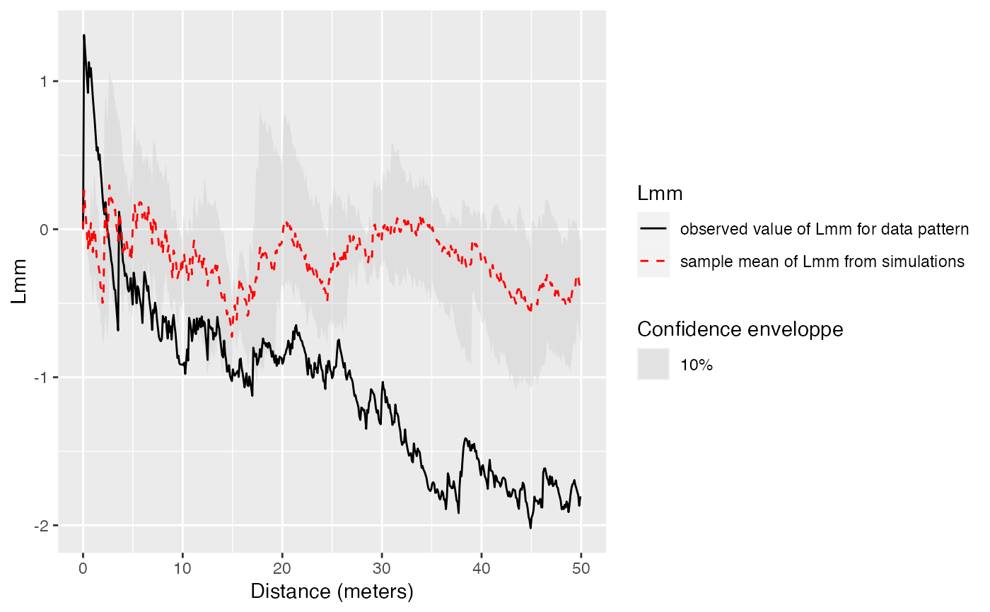
Estimation of the confidence envelope of the Lmm function under its null hypothesis

Simulates point patterns according to the null hypothesis and returns the envelope of Lmm according to the confidence level.

Usage

LmmEnvelope(X, r = NULL, NumberOfSimulations = 100, Alpha = 0.05,
            ReferenceType = "", Global = FALSE,
            verbose = interactive(), parallel = FALSE, parallel_pgb_refresh = 1/10)

Arguments

X

A weighted, marked, planar point pattern (wmppp.object).

r

A vector of distances. If NULL, a sensible default value is chosen (512 intervals, from 0 to half the diameter of the window) following spatstat.

NumberOfSimulations

The number of simulations to run, 100 by default.

Alpha

The risk level, 5% by default.

ReferenceType

One of the point types. Others are ignored. Default is all point types.

Global

Logical; if TRUE, a global envelope sensu Duranton and Overman (2005) is calculated.

verbose

Logical; if TRUE, print progress reports during the simulations.

parallel

Logical; if TRUE, simulations can be run in parallel, see details.

parallel_pgb_refresh

The proportion of simulations steps to be displayed by the parallel progress bar. 1 will show all but may slow down the computing, 1/100 only one out of a hundred.

Details

This envelope is local by default, that is to say it is computed separately at each distance. See Loosmore and Ford (2006) for a discussion.

The global envelope is calculated by iteration: the simulations reaching one of the upper or lower values at any distance are eliminated at each step. The process is repeated until Alpha / Number of simulations simulations are dropped. The remaining upper and lower bounds at all distances constitute the global envelope. Interpolation is used if the exact ratio cannot be reached.

Parallel simulations rely on the future and doFuture packages. Before calling the function with argument parallel = TRUE, you must choose a strategy and set it with plan. Their progress bar relies on the progressr package. They must be activated by the user by handlers.

Value

An envelope object (envelope). There are methods for print and plot for this class.

The fv contains the observed value of the function, its average simulated value and the confidence envelope.

References

Duranton, G. and Overman, H. G. (2005). Testing for Localisation Using Micro-Geographic Data. Review of Economic Studies 72(4): 1077-1106.

Kenkel, N. C. (1988). Pattern of Self-Thinning in Jack Pine: Testing the Random Mortality Hypothesis. Ecology 69(4): 1017-1024.

Loosmore, N. B. and Ford, E. D. (2006). Statistical inference using the G or K point pattern spatial statistics. Ecology 87(8): 1925-1931.

Marcon, E. and F. Puech (2017). A typology of distance-based measures of spatial concentration. Regional Science and Urban Economics. 62:56-67.

See also

Lmmhat

Examples

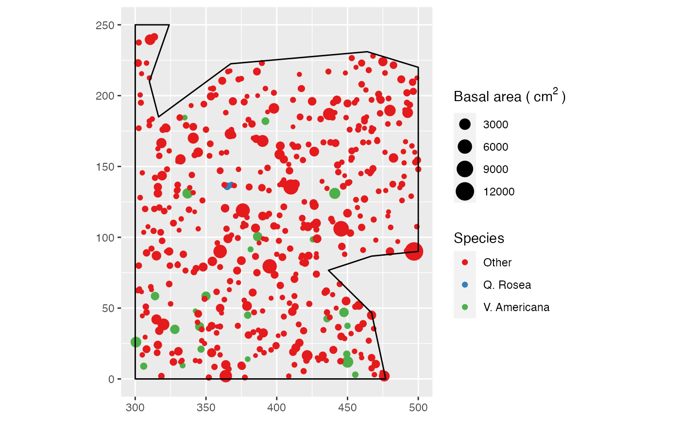
data(paracou16)
# Keep only 20% of points to run this example
X <- as.wmppp(rthin(paracou16, 0.2))
autoplot(X,
  labelSize = expression("Basal area (" ~cm^2~ ")"),
  labelColor = "Species")


# Calculate confidence envelope (should be 1000 simulations, reduced to 4 to save time)
r <- seq(0, 30, 2)
NumberOfSimulations <- 4
Alpha <- .10
autoplot(LmmEnvelope(X, r, NumberOfSimulations, Alpha))