Estimation of the density of neighbors
The function (Duranton and Overman 2005) is the probability density to find a neighbor a given distance apart from a point of interest in a finite point process. The function integrates the weights of points: it is the density probability to find an employee apart from an employee of interest. The function (Lang, Marcon, and Puech 2020) is the ratio of neighbors of interest at distance normalized by its value over the whole domain.
All those functions require smoothing the observed data: the
probability to find a neighbor exactly
apart from an arbitrary point is zero so neighbors around
apart are considered. The density function is used for that
purpose. It applies kernel density estimation. In
,
Gaussian kernels are used following Duranton and
Overman (2005). Actually, the important choice in kernel density
estimation is not the type of kernel but the bandwidth.
The bandwidth defines how close to the distance between two points must be to influence the estimation of the density at . A small bandwidth only considers the closest values so the estimation is close to the data. A large bandwidth considers more points and gives a smoother estimation.
Available algorithms
Duranton and Overman (2005), in the
original paper introducing the
function, used the optimal bandwidth according to Silverman (1986), i.e. the argument
bw = "nrd0" of function density. This is the
default choice in the functions of
,
i.e. the argument Original = TRUE in Kdhat,
mhat and similar functions.
A better choice may be Original = FALSE to apply the
estimation of Sheather and Jones (1991),
i.e. the argument bw = "SJ" of function
density, which has better theoretical support. The result
is usually less smoothed.
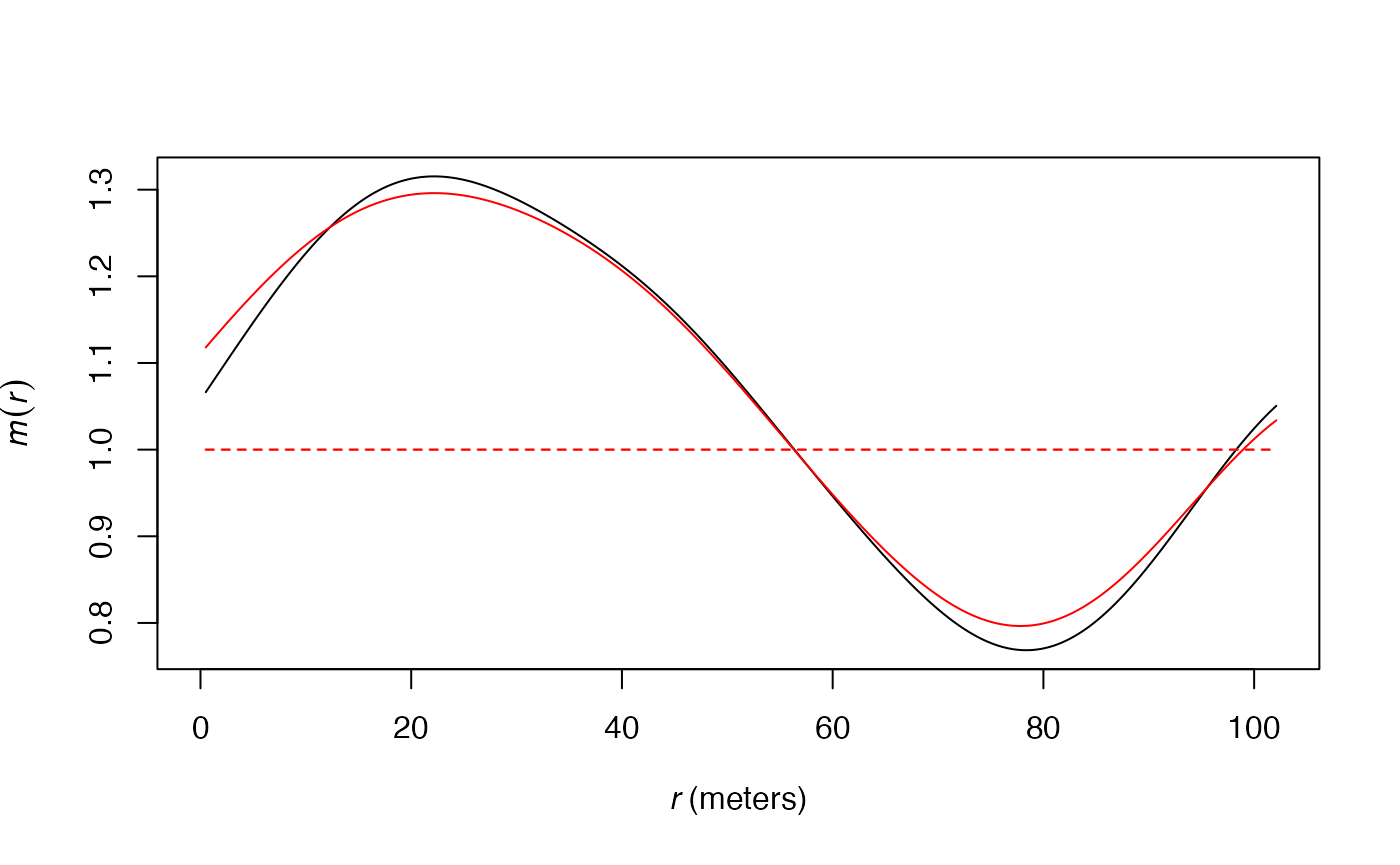
The following figure shows this difference on the estimation of the
function applied to the paracou16 point set: the red curve
is for the original estimation, the black one uses the Sheather and
Jones bandwidth.
## Loading required package: Rcpp## Loading required package: spatstat.explore## Loading required package: spatstat.data## Loading required package: spatstat.univar## spatstat.univar 3.1-3## Loading required package: spatstat.geom## spatstat.geom 3.4-1## Loading required package: spatstat.random## spatstat.random 3.4-1## Loading required package: nlme## spatstat.explore 3.4-3
# Sheather and Jones bandwidth in black
plot(
  mhat(
    paracou16,
    ReferenceType = "Q. Rosea",
    Original = FALSE
  ),
  main = "",
  legend = FALSE
)
# Original bandwidth in red
plot(
  mhat(
    paracou16,
    ReferenceType = "Q. Rosea"
  ),
  col = "red",
  main = "",
  add = TRUE
)
Data
The data used by those algorithms is the set of distances between
pairs of points. In
,
only pairs of points less than twice the maximum value of
are considered: very distant pairs of points are of little interest to
estimate functions based on the number of neighbors of points. With the
default arguments, almost all point pairs are included, except for the
most distant ones, i.e. more than two thirds of the window’s diameter
apart. If the user wants to focus on small distances, i.e. choose
much less than the default value, then the most distant point pairs
(more than twice the max value of
)
will be ignored, resulting in a smaller bandwidth and consequently a
more acute (less smoothed) estimation of the functions. The following
figure shows this effect on the estimation of the
function applied to the paracou16 point set. The default
distance range is used for the black curve. The red curve is the same
function estimated up to 30 meters only, resulting into a narrower
bandwith: the curve of
is less smoothed.
plot(
  Kdhat(
    paracou16,
    ReferenceType = "Q. Rosea",
    Original = FALSE
  ),
  ylim = c(0, 0.008),
  main = ""
)
plot(
  Kdhat(
    paracou16,
    r = 0:30,
    ReferenceType = "Q. Rosea",
    Original = FALSE
  ),
  main = "",
  col = "red",
  add = TRUE)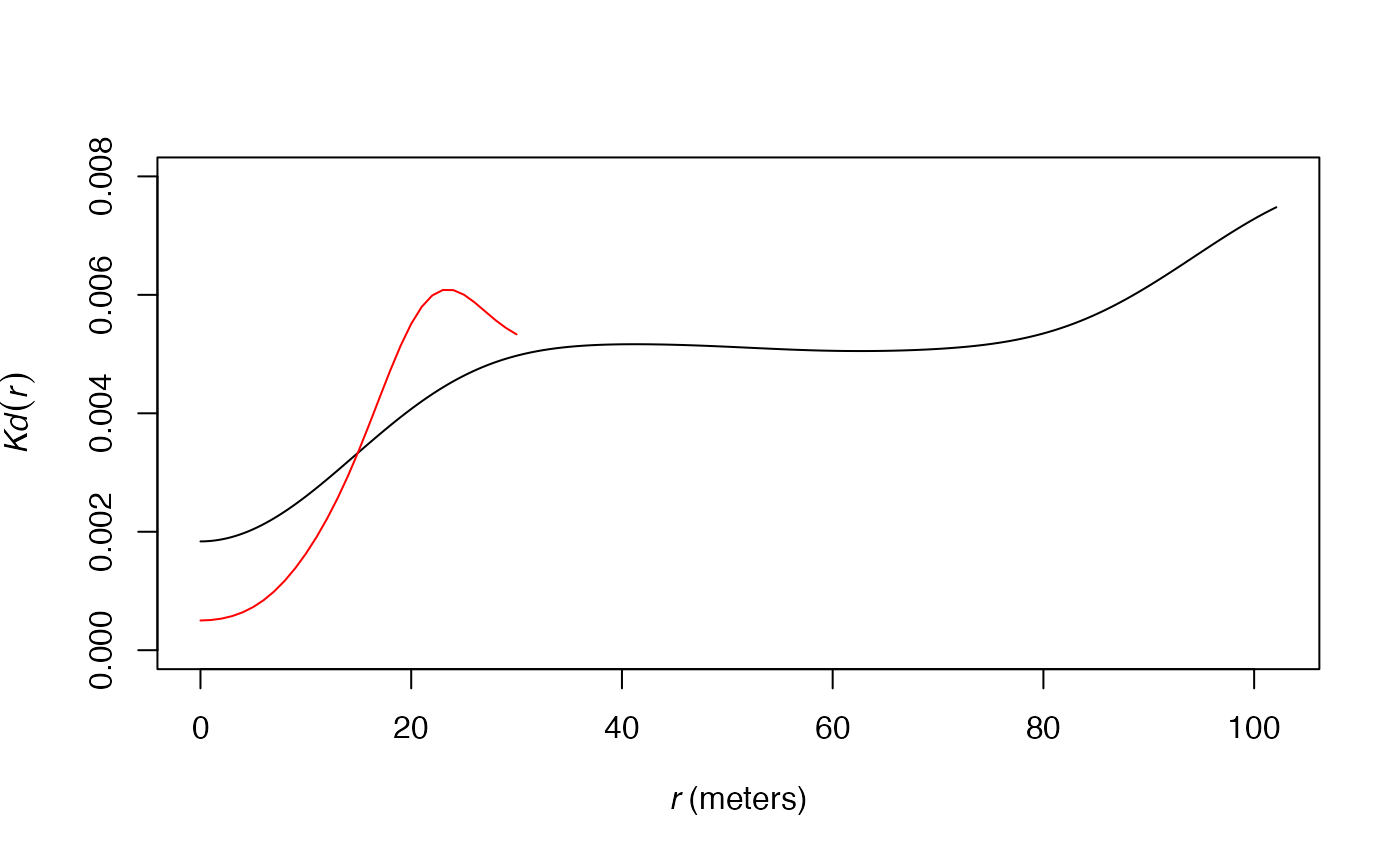
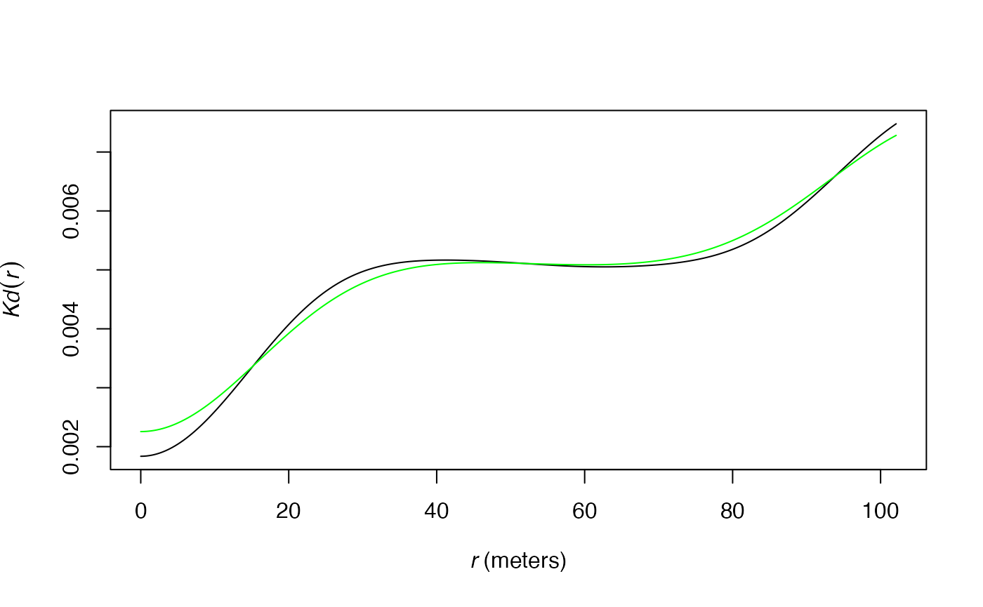
The approximated algorithm used to calculate
and
retains point pairs up to twice the max value of
and rounds their distances in 2048 (this number can be increased by the
Approximate argument) equally-spaced values. This set of
distances (actually, only those corresponding to at least a pair of
points) is used to choose the bandwidth. Simulations show that the
approximated algorithm yields bandwidths very similar to those obtained
by exact computation.
# Exact computation in black
plot(
  Kdhat(
    paracou16,
    ReferenceType = "Q. Rosea",
    Original = FALSE
  ),
  main = ""
)
# Approximated computation in green
plot(
  Kdhat(
    paracou16,
    ReferenceType = "Q. Rosea",
    Original = FALSE,
    Approximate = 1
  ),
  main = "",
  col = "green",
  add = TRUE
)
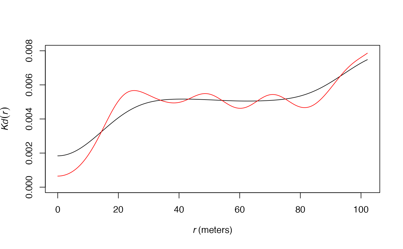
Fine tuning
The users can choose to multiply the bandwidth by argument
Adjust. Values over 1 will smooth the density estimation;
under 1, they will sharpen it.
# Default bandwith in black
plot(
  Kdhat(
    paracou16,
    ReferenceType = "Q. Rosea",
    Original = FALSE
  ),
  ylim = c(0, 0.008),
  main = ""
)
# Adjusted (half) bandwidth in red
plot(
  Kdhat(
    paracou16,
    ReferenceType = "Q. Rosea",
    Original = FALSE,
    Adjust = 1/2
  ),
  main = "",
  col = "red",
  add = TRUE
)
Conclusion
Density estimation heavily relies on the choice of its bandwidth. In
,
several choices influence its value. The first one is between the
original, i.e. following Duranton and Overman
(2005), and the more acute algorithm by Sheather and Jones (1991). Then, the distances
taken into account, i.e. the argument r (actually, its
maximum value) must be chosen carefully. A large r max
value increases the bandwidth since distant pair points are taken into
account. Decreasing r allows focusing on close neighbors: a
smaller bandwidth will be used and the function estimations will be less
smoothed, especially at small distances.
Last, the bandwidth can be arbitrarily modified by the
Adjust argument if necessary.
The default values of arguments (especially r) are a
good choice to obtain standard estimations of the
and
functions. If consistency with the original estimation of
by Duranton and Overman (2005) is not
important, Original = FALSE is even better. Whatever the
user’s choices, the bandwidth is chosen the same way for the estimation
of a distance-based function and its confidence envelope according to a
null hypothesis, allowing to detect departures of the oberved data from
the null hypothesis consistently.