Asymptotic Estimation, Interpolation and Extrapolation
Source:vignettes/articles/extrapolation.Rmd
extrapolation.RmdEstimation of diversity in divent relies on classical assumptions that are recalled here. The observed data is a sample of a community (or several communities if data is a metacommunity). All “reduced-bias estimator” are asymptotic estimators of the community diversity: if the sample size could be extended infinitely, diversity would tend to the diversity of the whole (asymptotic) community. In hyperdiverse ecosystems such as evergreen forests, the asymptotic community generally does not exist in the field because of environmental variations: increasing the size of the sample results in sampling in different communities. Thus, the asymptotic estimators of diversity correspond to theoretical asymptotic communities that do not necessarily exist. In other words, the asymptotic diversity is that of a community that would provide the observed sample.
Diversity is accumulated as a function of sample size. HCDT (aka Tsallis) entropy (thus Hill numbers and phylodiversity) can be estimated at any sample size (Chao et al. 2014), by interpolation down from the actual sample size and by extrapolation up to infinite sample size, i.e. the asymptotic estimator. Alternatively, sample size may be replaced by sample coverage, by interpolation from arbitrary small sample coverages to that of the actual sample, and by extrapolation up to the asymptotic estimator whose sample coverage is 1.
Asymptotic estimation
If community data is a vector of probabilities, sample size is unknown so the only available estimation is that of the actual sample.
library("dplyr")
library("divent")
# Paracou plot 6, subplot 1:
# 1,5 ha of tropical forest, distribution of probabilities
paracou_6_abd[1, ] %>%
  as_probabilities() %>%
  print() ->
  prob_paracou6_1
## # A tibble: 1 × 337
## site weight Abarema_jupunba Abarema_mataybifolia Amaioua_guianensis
## <chr> <dbl> <dbl> <dbl> <dbl>
## 1 subplot_1 1.56 0.00212 0.00212 0.00106
## # ℹ 332 more variables: Amanoa_congesta <dbl>, Amanoa_guianensis <dbl>,
## # Ambelania_acida <dbl>, Amphirrhox_longifolia <dbl>, Andira_coriacea <dbl>,
## # Apeiba_glabra <dbl>, Aspidosperma_album <dbl>, Aspidosperma_cruentum <dbl>,
## # Aspidosperma_excelsum <dbl>, Bocoa_prouacensis <dbl>,
## # Brosimum_guianense <dbl>, Brosimum_rubescens <dbl>, Brosimum_utile <dbl>,
## # Carapa_surinamensis <dbl>, Caryocar_glabrum <dbl>, Casearia_decandra <dbl>,
## # Casearia_javitensis <dbl>, Catostemma_fragrans <dbl>, …
# Diversity of order 1, no reduced-bias estimator available.
div_hill(prob_paracou6_1, q = 1)
## # A tibble: 1 × 5
## site weight estimator order diversity
## <chr> <dbl> <chr> <dbl> <dbl>
## 1 subplot_1 1.56 naive 1 77.0Further estimation requires abundances, i.e. the number of individuals per species. Then, the default estimator is the asymptotic one.
# Diversity of order 1, default asymptotic estimator used.
div_hill(paracou_6_abd[1, ], q = 1)
## # A tibble: 1 × 5
## site weight estimator order diversity
## <chr> <dbl> <chr> <dbl> <dbl>
## 1 subplot_1 1.56 UnveilJ 1 96.3Several asymptotic estimators are available in the literature and implemented in divent. For consistency, divent uses the jackknife estimator of richness and the unveiled jackknife estimator for entropy. The advantage of these estimators is that they provide reliable estimations even though the sampling effort is low: then, the estimation variance increases but its bias remains acceptable because the order of the jackknife estimator is chosen according to the data. Poorly-sampled communities are estimated by a higher-order jackknife, resulting in higher estimation variance.
For well-sampled communities, i.e. in the domain of validity of the jackknife of order 1, the Chao1 estimator of richness and the Chao-Jost estimator of entropy are the best choices because they have the best mathematical support, but they will severely underestimate the diversity of poorly-sampled communities. They also are more computer-intensive.
# Estimation of richness relies on jackknife 3 (poor sampling)
div_richness(paracou_6_abd[1, ])
## # A tibble: 1 × 5
## site weight estimator order diversity
## <chr> <dbl> <chr> <dbl> <dbl>
## 1 subplot_1 1.56 Jackknife 3 0 355
# Richness is underestimated by the Chao1 estimator
div_richness(paracou_6_abd[1, ], estimator = "Chao1")
## # A tibble: 1 × 5
## site weight estimator order diversity
## <chr> <dbl> <chr> <dbl> <dbl>
## 1 subplot_1 1.56 Chao1 0 290.
# Diversity of order 1 underestimated by the Chao-Jost estimator
div_hill(paracou_6_abd[1, ], q = 1, estimator = "ChaoJost")
## # A tibble: 1 × 5
## site weight estimator order diversity
## <chr> <dbl> <chr> <dbl> <dbl>
## 1 subplot_1 1.56 ChaoJost 1 91.3Choosing the estimation level
Asymptotic estimation is not always the best choice, for example when comparing the diversity of poorly-sampled communities: a lower sample coverage can be chosen to limit the uncertainty of estimation.
# Actual sample coverage
coverage(paracou_6_abd[1, ])
## # A tibble: 1 × 4
## site weight estimator coverage
## <chr> <dbl> <chr> <dbl>
## 1 subplot_1 1.56 ZhangHuang 0.911The estimation level may be a sample size or a sample coverage that is converted internally into a sample size.
# Diversity at half the sample size (interpolated)
paracou6_1_size <- abd_sum(paracou_6_abd[1, ], as_numeric = TRUE)
div_hill(paracou_6_abd[1, ], q = 1, level = round(paracou6_1_size / 2))
## # A tibble: 1 × 6
## site weight estimator order level diversity
## <chr> <dbl> <chr> <dbl> <dbl> <dbl>
## 1 subplot_1 1.56 Interpolation 1 471 67.6
# Sample size corresponding to 90% coverage
coverage_to_size(paracou_6_abd[1, ], sample_coverage = 0.9)
## # A tibble: 1 × 4
## site weight sample_coverage size
## <chr> <dbl> <dbl> <dbl>
## 1 subplot_1 1.56 0.9 819
# Diversity at 90% sample coverage
div_hill(paracou_6_abd[1, ], q = 1, level = 0.9)
## # A tibble: 1 × 6
## site weight estimator order level diversity
## <chr> <dbl> <chr> <dbl> <dbl> <dbl>
## 1 subplot_1 1.56 Interpolation 1 819 75.4If the sample size is smaller than the actual sample, entropy is interpolated.
If it is higher, entropy must be extrapolated. For diversity orders equal to 0 (richness), 1 (Shannon) or 2 (Simpson), explicit, almost unbiased estimators are used. Continuity of the estimation of diversity around the actual sample size is guaranteed.
# Simpson diversity at levels from 0.9 to 1.1 times the sample size
accum_hill(
  paracou_6_abd[1, ],
  q = 2,
  levels = round(0.9 * paracou6_1_size):round(1.1 * paracou6_1_size)) %>%
  autoplot()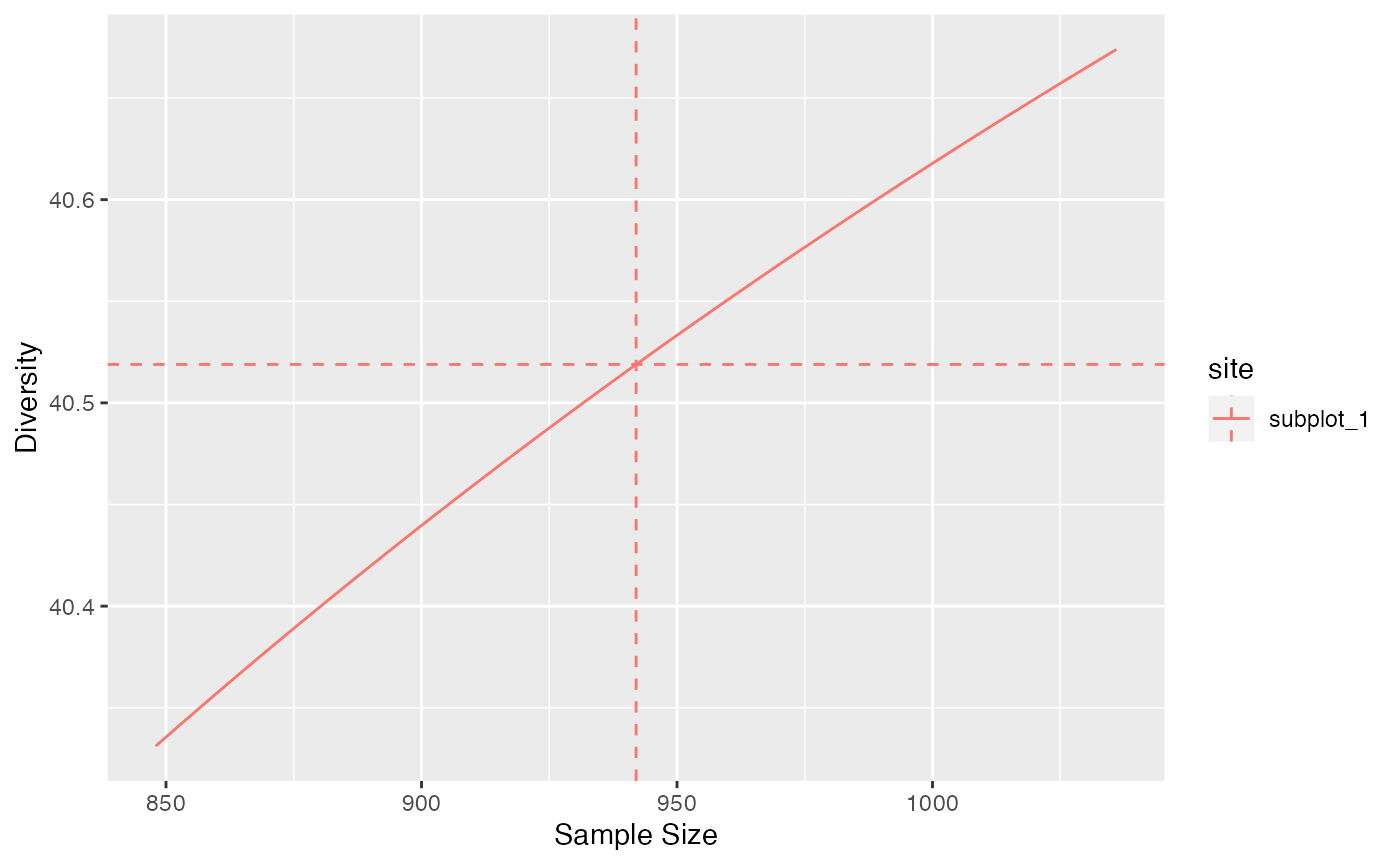
For non-integer orders, things get more complicated. In divent, asymptotic entropy is estimated by the unveiled jackknife estimator and rarefied down to the actual sample size. There is no reason for it to correspond exactly to the observed entropy. The asymptotic richness is the less robust part of the estimation thus it is adjusted iteratively until the rarefied entropy equals the actual sample’s entropy, ensuring continuity between interpolation and extrapolation.
The default arguments of all functions apply this strategy, except for Simpson’s diversity (\(q = 2\)) that is estimated directly without bias.
Diversity accumulation
Diversity Accumulation Curves (DAC) are a generalization of the well-known Species Accumulation Curves (SAC). They represent diversity as a function of sample size.
The accum_hill() function allows to build them. A
bootstrap confidence interval can be calculated around the estimated DAC
by simulating random multinomial draws of the asymptotic distribution at
each sample size.
# Diversity at levels from 1 to twice the sample size
accum_hill(
  paracou_6_abd[1, ],
  q = 1,
  levels = seq_len(1.1 * paracou6_1_size),
  n_simulations = 1000
) %>%
  autoplot()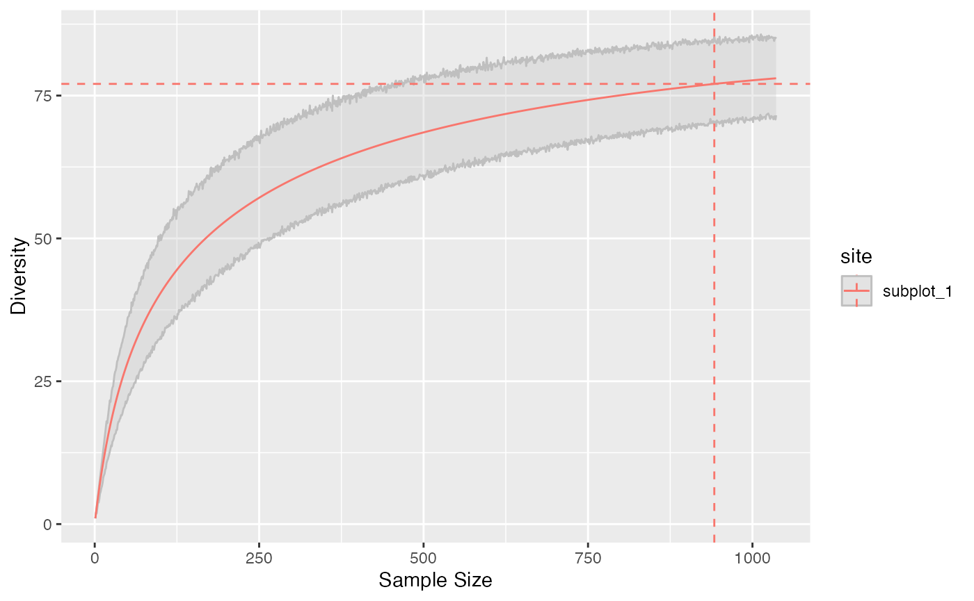
To ensure continuity of the DAC around the actual sample, the asymptotic diversity is estimated by unveiling the asymptotic distribution, choosing the number of species such that the rarefied diversity at the observed sample size is the observed diversity. This means that the extrapolated diversity at a high sample coverage will differ from the best asymptotic estimation, sometimes quite much if sampling level is poor.
# Extrapolation at 99.99% sample coverage
div_hill(paracou_6_abd[1, ], q = 1, level = 0.9999)
## # A tibble: 1 × 6
## site weight estimator order level diversity
## <chr> <dbl> <chr> <dbl> <dbl> <dbl>
## 1 subplot_1 1.56 Chao2015 1 8615 94.0
# Unveiled Jaccknife asymptotic estimator
div_hill(paracou_6_abd[1, ], q = 1)
## # A tibble: 1 × 5
## site weight estimator order diversity
## <chr> <dbl> <chr> <dbl> <dbl>
## 1 subplot_1 1.56 UnveilJ 1 96.3
# Chao-Jost estimator
div_hill(paracou_6_abd[1, ], q = 1, estimator = "ChaoJost")
## # A tibble: 1 × 5
## site weight estimator order diversity
## <chr> <dbl> <chr> <dbl> <dbl>
## 1 subplot_1 1.56 ChaoJost 1 91.3Diversity profiles at a sampling level
Diversity profiles are usually asymptotic but they can be calculated at any coverage of sampling level.
# Diversity at levels from 1 to twice the sample size
profile_hill(paracou_6_abd[1, ], level = paracou6_1_size * 1.5) %>%
  autoplot()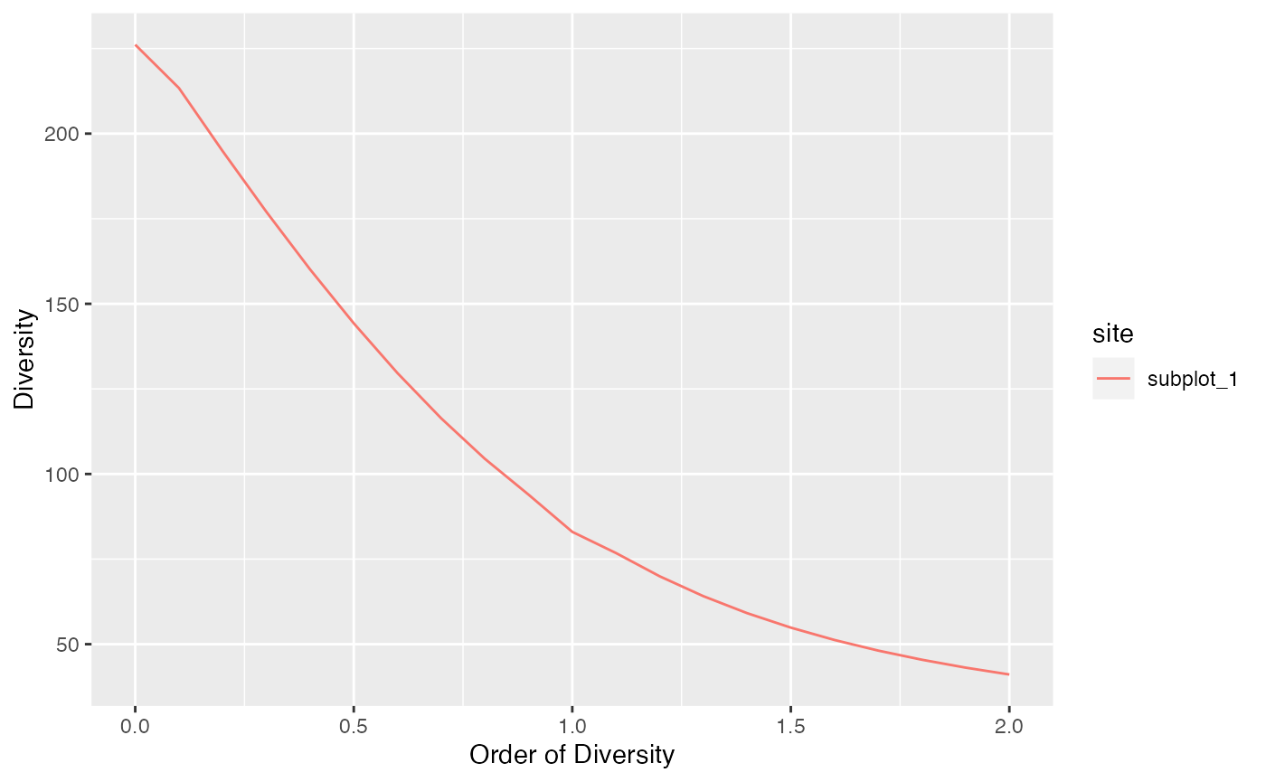
Extrapolated diversity is estimated at each order such that it is continuous at the observed sample size.
Differences with the iNEXT package
iNEXT (Hsieh et al. 2016) is
designed primarily to interpolate or extrapolate diversity of integer
orders. Extrapolation of diversity of order 0 relies on the Chao1
estimator of richness and that of order 1 uses the Chao-Jost estimator.
In divent, extrapolation relies on the estimation of the
asymptotic distribution of the community with asymptotic richness such
that the entropy of the asymptotic distribution rarefied to the observed
sample size equals the observed entropy of the data. This approach
allows consistent estimation of extrapolated diversity at integer and
non-integer orders, thus allowing consistent diversity profiles without
discontinuities at \(q = 0\) and \(q = 1\). The results of iNEXT can
be obtained by forcing argument estimator = "ChaoJost".
library("iNEXT")
data(spider)
# Extrapolated diversity of an example dataset
estimateD(spider$Girdled, level = 300)
## Assemblage m Method Order.q SC qD qD.LCL qD.UCL
## 1 data 300 Extrapolation 0 0.9579518 33.317733 25.804082 40.831384
## 2 data 300 Extrapolation 1 0.9579518 12.869603 10.314593 15.424612
## 3 data 300 Extrapolation 2 0.9579518 7.983882 5.993923 9.973841
# Similar estimation by divent
div_hill(spider$Girdled, q = 0, level = 300, estimator = "ChaoJost")
## # A tibble: 1 × 4
## estimator order level diversity
## <chr> <dbl> <dbl> <dbl>
## 1 jackknife 0 300 33.5
div_hill(spider$Girdled, q = 1, level = 300, estimator = "ChaoJost")## # A tibble: 1 × 4
## estimator order level diversity
## <chr> <dbl> <dbl> <dbl>
## 1 Chao2015 1 300 13.1
# Estimation at order 2 is explicit, with no optional choice
div_hill(spider$Girdled, q = 2, level = 300)
## # A tibble: 1 × 4
## estimator order level diversity
## <chr> <dbl> <dbl> <dbl>
## 1 Chao2014 2 300 7.98
# Default estimation of divent
div_hill(spider$Girdled, q = 0, level = 300)
## # A tibble: 1 × 4
## estimator order level diversity
## <chr> <dbl> <dbl> <dbl>
## 1 jackknife 0 300 33.5
div_hill(spider$Girdled, q = 1, level = 300)## # A tibble: 1 × 4
## estimator order level diversity
## <chr> <dbl> <dbl> <dbl>
## 1 Chao2015 1 300 13.1Small differences are due to different estimators of sample coverage:
divent uses the more accurate ZhangHuang estimator
by default.
Last, confidence intervals of diversity accumulation assume normality in iNEXT: estimation variance is estimated by bootstrap and the confidence interval is defined as \(\pm 1.96\) times the standard deviation. In divent, confidence intervals are built directly from the quantiles of bootstrapped estimations.