Estimation of the D function
Dhat.RdEstimates the D function
Arguments
- X
A weighted, marked, planar point pattern (
wmppp.object).- r
A vector of distances. If
NULL, a sensible default value is chosen (512 intervals, from 0 to half the diameter of the window) following spatstat.- Cases
One of the point types.
- Controls
One of the point types. If
NULL, controls are all types except for cases.- Intertype
Logical; if
TRUE, D is computed as Di in Marcon and Puech (2012).- CheckArguments
Logical; if
TRUE, the function arguments are verified. Should be set toFALSEto save time in simulations for example, when the arguments have been checked elsewhere.
Details
The Di function allows comparing the structure of the cases to that of the controls around cases, that is to say the comparison is made around the same points. This has been advocated by Arbia et al. (2008) and formalized by Marcon and Puech (2012).
References
Arbia, G., Espa, G. and Quah, D. (2008). A class of spatial econometric methods in the empirical analysis of clusters of firms in the space. Empirical Economics 34(1): 81-103.
Diggle, P. J. and Chetwynd, A. G. (1991). Second-Order Analysis of Spatial Clustering for Inhomogeneous Populations. Biometrics 47(3): 1155-1163.
Marcon, E. and F. Puech (2017). A typology of distance-based measures of spatial concentration. Regional Science and Urban Economics. 62:56-67.
Examples
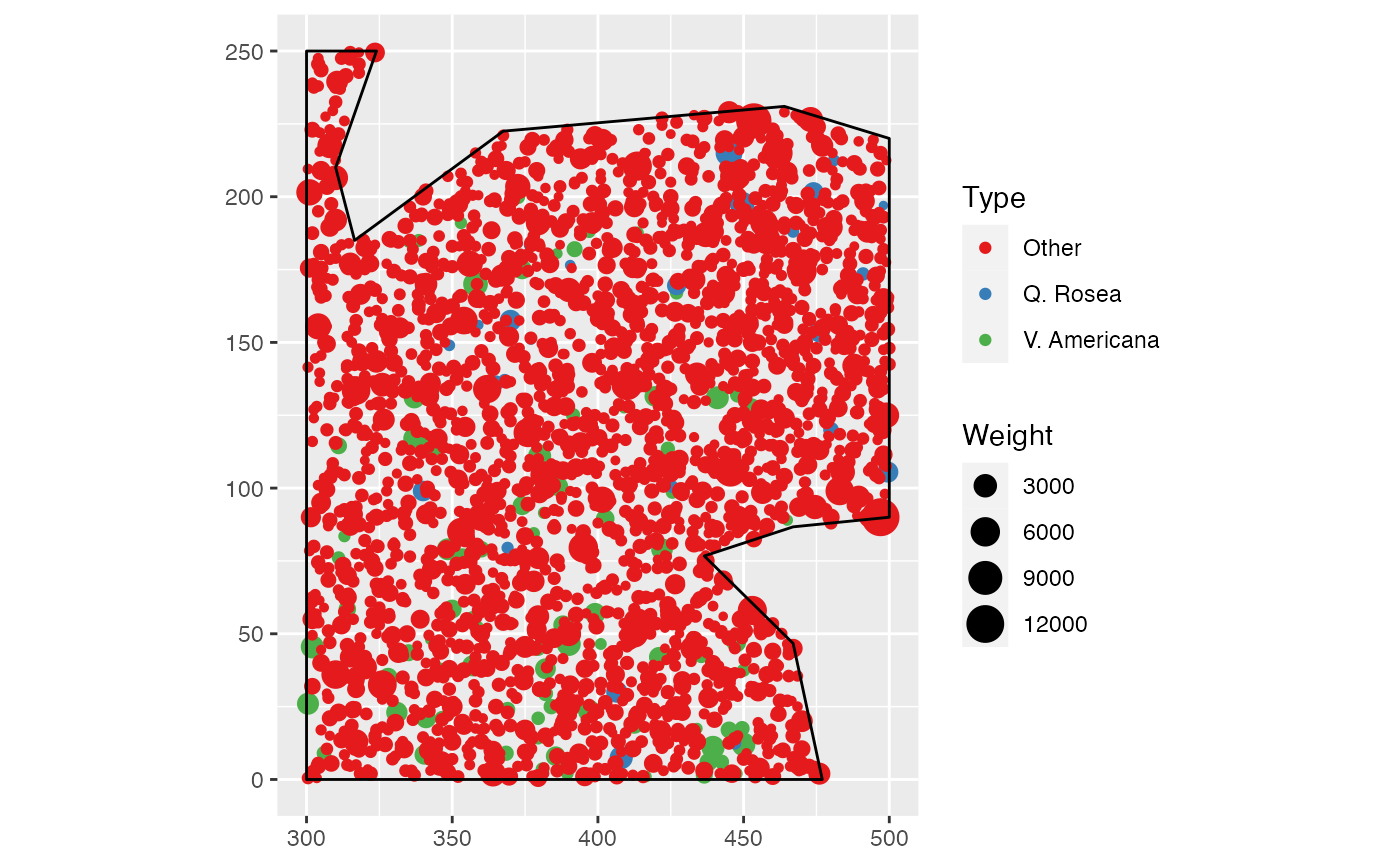
data(paracou16)
autoplot(paracou16)
 # Calculate D
r <- 0:30
(Paracou <- Dhat(paracou16, r, "V. Americana", "Q. Rosea", Intertype = TRUE))
#> Function value object (class ‘fv’)
#> for the function r -> D(r)
#> ................................................................
#> Math.label Description
#> r r distance argument r
#> theo D[theo](r) theoretical Poisson D(r)
#> iso hat(D)[iso](r) Ripley isotropic correction estimate of D(r)
#> ................................................................
#> Default plot formula: .~r
#> where “.” stands for ‘theo’, ‘iso’
#> Recommended range of argument r: [0, 30]
#> Available range of argument r: [0, 30]
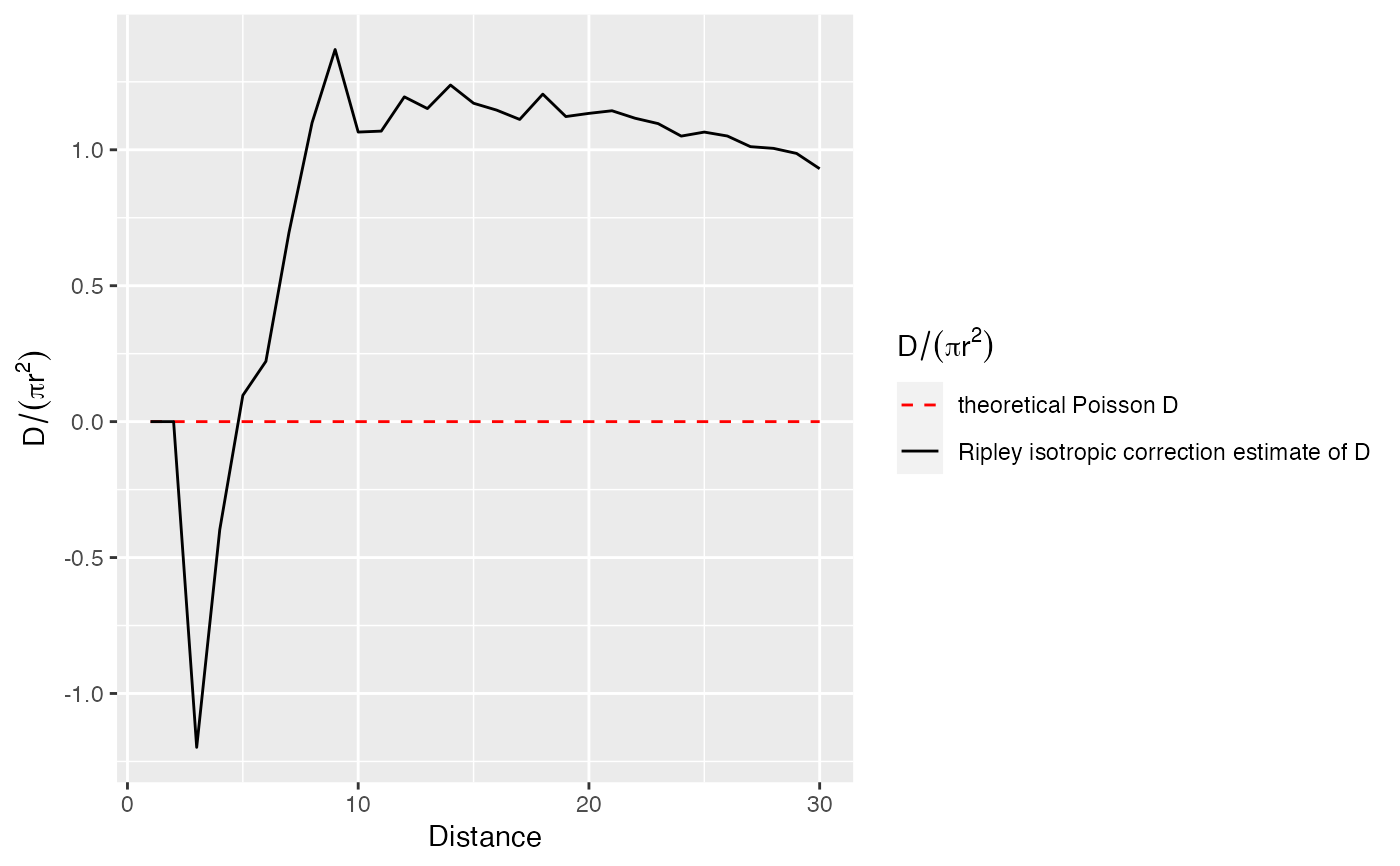
# Plot (after normalization by pi.r^2)
autoplot(Paracou, ./(pi*r^2) ~ r)
# Calculate D
r <- 0:30
(Paracou <- Dhat(paracou16, r, "V. Americana", "Q. Rosea", Intertype = TRUE))
#> Function value object (class ‘fv’)
#> for the function r -> D(r)
#> ................................................................
#> Math.label Description
#> r r distance argument r
#> theo D[theo](r) theoretical Poisson D(r)
#> iso hat(D)[iso](r) Ripley isotropic correction estimate of D(r)
#> ................................................................
#> Default plot formula: .~r
#> where “.” stands for ‘theo’, ‘iso’
#> Recommended range of argument r: [0, 30]
#> Available range of argument r: [0, 30]
# Plot (after normalization by pi.r^2)
autoplot(Paracou, ./(pi*r^2) ~ r)