2 Use R

The literature devoted to learning R is flourishing. The following books are an arbitrary but useful selection:

• R for Data Science (Wickham and Grolemund 2016) presents a complete working method, consistent with the tidyverse.
• Advanced R (Wickham 2014) is the reference for mastering the subtleties of the language and understanding how R works.
• Finally, Efficient R programming (Gillespie and Lovelace 2016) deals with code optimization.

Some advanced aspects of coding are seen here. Details on the different languages of R are useful for creating packages. The environments are presented next, for the proper understanding of the search for objects called by the code. Finally, the optimization of code performance is discussed in depth (loops, C++ code and parallelization) and illustrated by a case study.

2.1 The languages of R

R includes several programming languages. The most common is S3, but it is not the only one¹⁸.

2.1.1 Base

The core of R is the primitive functions and basic data structures like the sum function and matrix data:

pryr::otype(sum)

## [1] "base"

typeof(sum)

## [1] "builtin"

pryr::otype(matrix(1))

## [1] "base"

typeof(matrix(1))

## [1] "double"

The pryr package allows to display the language in which objects are defined. The typeof() function displays the internal storage type of the objects:

• the sum() function belongs to the basic language of R and is a builtin function.
• the elements of the numerical matrix containing a single 1 are double precision reals, and the matrix itself is defined in the basic language.

Primitive functions are coded in C and are very fast. They are always available, whatever the packages loaded. Their use is therefore to be preferred.

2.1.2 S3

S3 is the most used language, often the only one known by R users.

It is an object-oriented language in which classes, i.e. the type of objects, are declarative.

MyFirstName <- "Eric"
class(MyFirstName) <- "FirstName"

The variable MyFirstName is here classed as FirstName by a simple declaration.

Unlike the way a classical object-oriented language works¹⁹, S3 methods are related to functions, not objects.

# Default display
MyFirstName

## [1] "Eric"
## attr(,"class")
## [1] "FirstName"

print.Firstname <- function(x) cat("The first name is", x)
# Modified display
MyFirstName

## [1] "Eric"
## attr(,"class")
## [1] "FirstName"

In this example, the print() method applied to the “Firstname” class is modified. In a classical object-oriented language, the method would be defined in the class Firstname. In R, methods are defined from generic methods.

print is a generic method (“a generic”) declared in base.

pryr::otype(print)

## [1] "base"

Its code is just a UseMethod("print") declaration:

print

## function (x, ...) 
## UseMethod("print")
## <bytecode: 0x7fb89ff9fac8>
## <environment: namespace:base>

There are many S3 methods for print:

head(methods("print"))

## [1] "print.acf"               "print.activeConcordance"
## [3] "print.AES"               "print.all_vars"         
## [5] "print.anova"             "print.any_vars"

Each applies to a class. print.default is used as a last resort and relies on the type of the object, not its S3 class.

typeof(MyFirstName)

## [1] "character"

pryr::otype(MyFirstName)

## [1] "S3"

An object can belong to several classes, which allows a form of inheritance of methods. In a classical object oriented language, inheritance allows to define more precise classes (“FrenchFirstName”) which inherit from more general classes (“FirstName”) and thus benefit from their methods without having to redefine them. In R, inheritance is simply declaring a vector of increasingly broad classes for an object:

# Definition of classes by a vector
class(MyFirstName) <- c("FrenchFirstName", "FirstName")
# Alternative code, with inherits()
inherits(MyFirstName, what = "FrenchFirstName")

## [1] TRUE

inherits(MyFirstName, what = "FirstName")

## [1] TRUE

The generic looks for a method for each class, in the order of their declaration.

print.FrenchFirstName <- function(x) cat("French first name:",
    x)
MyFirstName

## French first name: Eric

In summary, S3 is the common language of R. Almost all packages are written in S3. Generics are everywhere but go unnoticed, for example in packages:

library("entropart")
.S3methods(class = "SpeciesDistribution")

## [1] autoplot plot    
## see '?methods' for accessing help and source code

The .S3methods() function displays all available methods for a class, as opposed to methods() which displays all classes for which the method passed as an argument is defined.

Many primitive functions in R are generic methods. To find out about them, use the help(InternalMethods) helper.

2.1.3 S4

S4 is an evolution of S3 that structures classes to get closer to a classical object oriented language:

• Classes must be explicitly defined, not simply declared.
• 1ttributes (i.e. variables describing objects), called slots, are explicitly declared.
• The constructor, i.e. the method that creates a new instance of a class (i.e. a variable containing an object of the class), is explicit.

Using the previous example, the S4 syntax is as follows:

# Definition of the class Person, with its slots
setClass("Person",  
         slots = list(LastName = "character", FirstName = "character"))
#  Construction of an instance
Me <- new("Person", LastName = "Marcon", FirstName = "Eric")
# Langage
pryr::otype(Me)

## [1] "S4"

Methods always belong to functions. They are declared by the setMethod() function:

setMethod("print", signature = "Person", function(x, ...) {
    cat("The person is:", x@FirstName, x@LastName)
})
print(Me)

## The person is: Eric Marcon

The attributes are called by the syntax variable@slot.

In summary, S4 is more rigorous than S3. Some packages on CRAN : Matrix, sp, odbc… and many on Bioconductor are written in S4 but the language is now clearly abandoned in favor of S3, notably because of the success of the tidyverse.

2.1.4 RC

RC was introduced in R 2.12 (2010) with the methods package.

Methods belong to classes, as in C++: they are declared in the class and called from the objects.

library("methods")
# Declaration of the class
PersonRC <- setRefClass("PersonRC", 
    fields = list(LastName = "character", FirstName = "character"),
    methods = list(print = function() cat(FirstName, LastName)))
# Constructeur
MeRC <- new("PersonRC", LastName = "Marcon", FirstName ="Eric")
# Language
pryr::otype(MeRC)

## [1] "RC"

# Call the print method
MeRC$print()

## Eric Marcon

RC is a confidential language, although it is the first “true” object-oriented language of R.

2.1.5 S6

S6²⁰ enhances RC but is not included in R: it requires installing its package.

Attributes and methods can be public or private. An initialize() method is used as a constructor.

library("R6")
PersonR6 <- R6Class("PersonR6", public = list(LastName = "character",
    FirstName = "character", initialize = function(LastName = NA,
        FirstName = NA) {
        self$LastName <- LastName
        self$FirstName <- FirstName
    }, print = function() cat(self$FirstName, self$LastName)))
MeR6 <- PersonR6$new(LastName = "Marcon", FirstName = "Eric")
MeR6$print()

## Eric Marcon

S6 allows to program rigorously in object but is very little used. The performances of S6 are much better than those of RC but are inferior to those of S3²¹.

The non-inclusion of R6 to R is shown by pryr:

pryr::otype(MeR6)

## [1] "S3"

2.1.6 Tidyverse

The tidyverse is a set of coherent packages that have evolved the way R is programmed. The set of essential packages can be loaded by the tidyverse package which has no other use:

library("tidyverse")

This is not a new language per se but rather an extension of S3, with deep technical modifications, notably the unconventional evaluation of expressions²², which it is not essential to master in detail.

Its principles are written in a manifesto²³. Its most visible contribution for the user is the sequence of commands in a flow (code pipeline).

In standard programming, the sequence of functions is written by successive nesting, which makes it difficult to read, especially when arguments are needed:

# Base-2 logarithm of the mean of 100 random numbers in a
# uniform distribution
log(mean(runif(100)), base = 2)

## [1] -1.127903

In the tidyverse, the functions are chained together, which often better matches the programmer’s thinking about data processing:

# 100 random numbers in a uniform distribution
runif(100) %>% 
  # Mean
  mean %>% 
  # Base-2 logarithm
  log(base=2)

## [1] -0.9772102

The pipe %>% is an operator that calls the next function by passing it as first argument the result of the previous function. Additional arguments are passed normally: for the readability of the code, it is essential to name them. Most of the R functions can be used without difficulty in the tidyverse, even though they were not designed for this purpose: it is sufficient that their first argument is the data to be processed.

The pipeline allows only one value to be passed to the next function, which prohibits multidimensional functions, such as f(x,y). The preferred data structure is the tibble, which is an improved dataframe: its print() method is more readable, and it corrects some unintuitive dataframe behavior, such as the automatic conversion of single-column dataframes to vectors. The columns of the dataframe or tibble allow to pass as much data as needed.

Finally, data visualization is supported by ggplot2 which relies on a theoretically sound graph grammar (Wickham 2010). Schematically, a graph is constructed according to the following model:

ggplot(data = <DATA>) + 
  <GEOM_FUNCTION>(
     mapping = aes(<MAPPINGS>),
     stat = <STAT>, 
     position = <POSITION>
  ) +
  <COORDINATE_FUNCTION> +
  <FACET_FUNCTION>

• The data is necessarily a dataframe.
• The geometry is the type of graph chosen (points, lines, histograms or other).
• The aesthetics (function aes()) designates what is represented: it is the correspondence between the columns of the dataframe and the elements necessary for the geometry.
• Statistics is the treatment applied to the data before passing it to the geometry (often “identity”, i.e. no transformation but “boxplot” for a boxplot). The data can be transformed by a scale function, such as scale_y_log10().
• The position is the location of the objects on the graph (often “identity”; “stack” for a stacked histogram, “jitter” to move the overlapping points slightly in a geom_point).
• The coordinates define the display of the graph (coord_fixed() to avoid distorting a map for example).
• Finally, facets offer the possibility to display several aspects of the same data by producing one graph per modality of a variable.

The set formed by the pipeline and ggplot2 allows complex processing in a readable code. Figure 2.1 shows the result of the following code:

# Diamonds data provided by ggplot2
diamonds %>% 
  # Keep only diamonds larger than half a carat
  filter(carat > 0.5) %>% 
  # Graph: price vs. weight
  ggplot(aes(x = carat, y = price)) +
    # Scatter plot
    geom_point() + 
    # Logarithmic scale
    scale_x_log10() + 
    scale_y_log10() + 
    # Linear regression
    geom_smooth(method = "lm")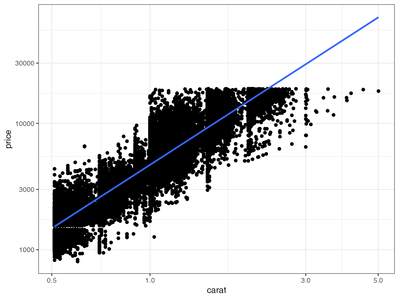

Figure 2.1: Price of diamonds according to their weight. Demonstration of the ggplot2 code combined with tidyverse data processing.

In this figure, two geometries (scatterplot and linear regression) share the same aesthetics (price vs. weight in carats) which is therefore declared upstream, in the ggplot() function.

The tidyverse is documented in detail in Wickham and Grolemund (2016) and ggplot2 in Wickham (2017).

2.2 Environments

R’s objects, data and functions, are named. Since R is modular, with the ability to add any number of packages to it, it is very likely that name conflicts will arise. To deal with them, R has a rigorous system of name precedence: code runs in a defined environment, inheriting from parent environments.

2.2.1 Organization

R starts in an empty environment. Each loaded package creates a child environment to form a stack of environments, of which each new element is called a “child” of the previous one, which is its “parent”.

The console is in the global environment, the child of the last loaded package.

search()

##  [1] ".GlobalEnv"        "package:R6"       
##  [3] "package:entropart" "package:lubridate"
##  [5] "package:forcats"   "package:stringr"  
##  [7] "package:dplyr"     "package:purrr"    
##  [9] "package:readr"     "package:tidyr"    
## [11] "package:tibble"    "package:ggplot2"  
## [13] "package:tidyverse" "package:stats"    
## [15] "package:graphics"  "package:grDevices"
## [17] "package:utils"     "package:datasets" 
## [19] "package:methods"   "Autoloads"        
## [21] "package:base"

The code of a function called from the console runs in a child environment of the global environment:

# Current environment
environment()

## <environment: R_GlobalEnv>

# The function f displays its environment
f <- function() environment()
# Display the environment of the function
f()

## <environment: 0x7fb88c67b118>

# Parent environment of the function's environment
parent.env(f())

## <environment: R_GlobalEnv>

2.2.2 Search

The search for ab object starts in the local environment. If it is not found, it is searched in the parent environment, then in the parent of the parent, until the environments are exhausted, which generates an error indicating that the object was not found.

Example:

# Variable q defined in the global environment
q <- "GlobalEnv"
# Function defining q in its environment
qLocalFunction <- function() {
    q <- "Function"
    return(q)
}
# The local variable is returned
qLocalFunction()

## [1] "Function"

# Poorly written function using a variable it does not
# define
qGlobalEnv <- function() {
    return(q)
}
# The global environment variable is returned
qGlobalEnv()

## [1] "GlobalEnv"

# Delete this variable
rm(q)
# The function base::q is returned
qGlobalEnv()

## function (save = "default", status = 0, runLast = TRUE) 
## .Internal(quit(save, status, runLast))
## <bytecode: 0x7fb8a5f980b0>
## <environment: namespace:base>

The variable q is defined in the global environment. The function qLocalFunction defines its own variable q. Calling the function returns the its local value because it is in the function’s environment.

The qGlobalEnv function returns the q variable that it does not define locally. So it looks for it in its parent environment and finds the variable defined in the global environment. By removing the variable from the global environment with rm(q), the qGlobalEnv() function scans the stack of environments until it finds an object named q in the base package, which is the function to exit R. It could have found another object if a package containing a q object had been loaded.

To avoid this erratic behavior, a function should never call an object not defined in its own environment.

2.2.3 Package namespaces

It is time to define precisely what packages make visible. Packages contain objects (functions and data) which they export or not. They are usually called by the library() function, which does two things:

• It loads the package into memory, allowing access to all its objects with the syntax package::object for exported objects and package:::object for non-exported ones.
• It then attaches the package, which places its environment on top of the stack.

It is possible to detach a package with the unloadNamespace() function to remove it from the environment stack. Example:

# entropart loaded and attached
library("entropart")
# is it attached?
isNamespaceLoaded("entropart")

## [1] TRUE

# stack of environments
search()

##  [1] ".GlobalEnv"        "package:R6"       
##  [3] "package:entropart" "package:lubridate"
##  [5] "package:forcats"   "package:stringr"  
##  [7] "package:dplyr"     "package:purrr"    
##  [9] "package:readr"     "package:tidyr"    
## [11] "package:tibble"    "package:ggplot2"  
## [13] "package:tidyverse" "package:stats"    
## [15] "package:graphics"  "package:grDevices"
## [17] "package:utils"     "package:datasets" 
## [19] "package:methods"   "Autoloads"        
## [21] "package:base"

# Diversity(), a function exported by entropart is found
Diversity(1, CheckArguments = FALSE)

## None 
##    1

# Detach and unload entropart
unloadNamespace("entropart")
# Is it attached?
isNamespaceLoaded("entropart")

## [1] FALSE

# Stack of environments, without entropart
search()

##  [1] ".GlobalEnv"        "package:R6"       
##  [3] "package:lubridate" "package:forcats"  
##  [5] "package:stringr"   "package:dplyr"    
##  [7] "package:purrr"     "package:readr"    
##  [9] "package:tidyr"     "package:tibble"   
## [11] "package:ggplot2"   "package:tidyverse"
## [13] "package:stats"     "package:graphics" 
## [15] "package:grDevices" "package:utils"    
## [17] "package:datasets"  "package:methods"  
## [19] "Autoloads"         "package:base"

# Diversity() cannot be found
tryCatch(Diversity(1), error = function(e) print(e))

## <simpleError in Diversity(1): could not find function "Diversity">

# but can be called with its full name
entropart::Diversity(1, CheckArguments = FALSE)

## None 
##    1

Calling entropart::Diversity() loads the package (i.e., implicitly executes loadNamespace("entropart")) but does not attach it.

In practice, one should limit the number of attached packages to limit the risk of calling an unwanted function, homonymous to the desired function. In critical cases, the full name of the function should be used: package::function().

A common issue occurs with the filter() function of dplyr, which is the namesake of the stats function. The stats package is usually loaded before dplyr, a package in the tidyverse. Thus, stats::filter() must be called explicitly.

However, the dplyr or tidyverse package (which attaches all the tidyverse packages) can be loaded systematically by creating a .RProfile at the root of the project containing the command:

library("tidyverse")

In this case, dplyr is loaded before stats so its function is inaccessible.

2.3 Measuring execution time

The execution time of long code can be measured very simply by the system.time command. For very short execution times, it is necessary to repeat the measurement: this is the purpose of the microbenchmark package.

2.3.1 system.time

The function returns the execution time of the code.

# Mean absolute deviation of 1000 values in a uniform
# distribution, repeated 100 times
system.time(for (i in 1:100) mad(runif(1000)))

##    user  system elapsed 
##   0.013   0.001   0.013

2.3.2 microbenchmark

The microbenchmark package is the most advanced.

The goal is to compare the speed of computing the square of a vector (or a number) by multiplying it by itself (\(x \times x\)) or by raising it to the power of 2 (\(x^2\)).

# Functions to test
f1 <- function(x) x * x
f2 <- function(x) x^2
f3 <- function(x) x^2.1
f4 <- function(x) x^3
# Initialization
X <- rnorm(10000)
# Test
library("microbenchmark")
(mb <- microbenchmark(f1(X), f2(X), f3(X), f4(X)))

## Unit: microseconds
##   expr     min      lq      mean   median       uq      max
##  f1(X)  27.955  29.006  38.75935  29.5940  30.6185  863.881
##  f2(X)  39.267  40.211  50.25438  40.7585  41.6150  885.665
##  f3(X) 245.083 246.150 257.01353 246.5975 247.3380 1082.756
##  f4(X) 309.997 314.961 327.47396 315.5495 317.0790 1278.603
##  neval
##    100
##    100
##    100
##    100

The returned table contains the minimum, median, mean, max and first and third quartile times, as well as the number of repetitions. The median value is to be compared. The number of repetitions is by default 100, to be modulated (argument times) according to the complexity of the calculation.

The test result, a microbenchmark object, is a raw table of execution times. The statistical analysis is done by the print and summary methods. To choose the columns to display, use the following syntax:

summary(mb)[, c("expr", "median")]

##    expr   median
## 1 f1(X)  29.5940
## 2 f2(X)  40.7585
## 3 f3(X) 246.5975
## 4 f4(X) 315.5495

To make calculations on these results, we must store them in a variable. To prevent the results from being displayed in the console, the simplest solution is to use the capture.output function by assigning its result to a variable.

dummy <- capture.output(mbs <- summary(mb))

The previous test is displayed again.

summary(mb)[, c("expr", "median")]

##    expr   median
## 1 f1(X)  29.5940
## 2 f2(X)  40.7585
## 3 f3(X) 246.5975
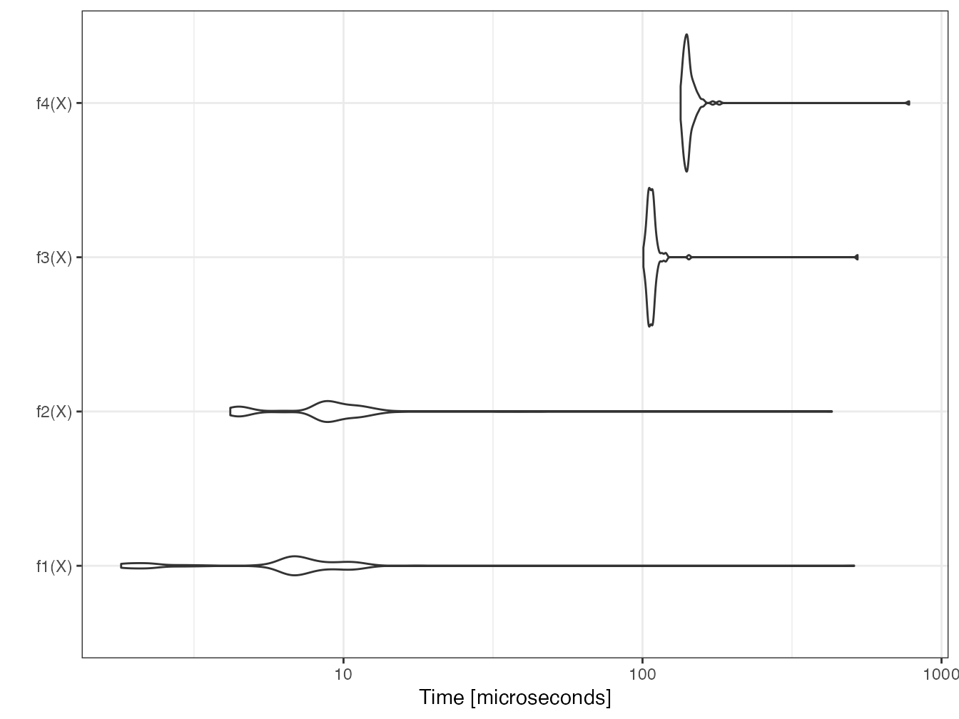
## 4 f4(X) 315.5495

The computation time is about the same between \(x \times x\) and \(x^2\). The power calculation is much longer, especially if the power is not integer, because it requires a logarithm calculation. The computation of the power 2 is therefore optimized by R to avoid the use of log.

Two graphical representations are available: the violins represent the probability density of the execution time; the boxplots are classical.

library("ggplot2")
autoplot(mb)

boxplot(mb)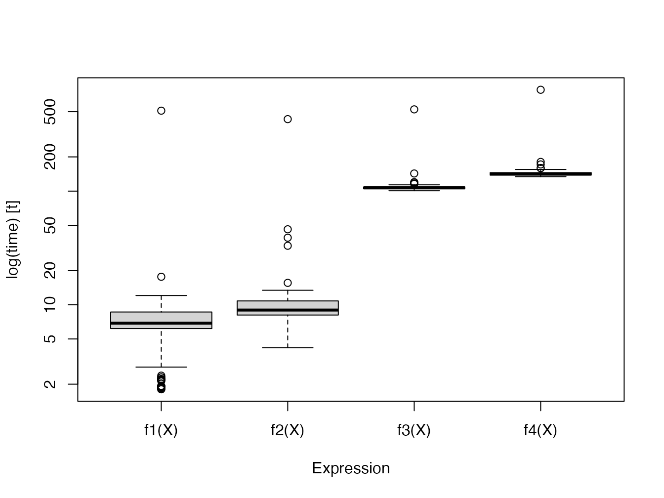

2.3.3 Profiling

profvis is RStudio’s profiling tool.

It tracks the execution time of each line of code and the memory used. The goal is to detect slow code portions that need to be improved.

library(profvis)
p <- profvis({
    # Cosine calculations
    cos(runif(10^7))
    # 1/2 second pause
    pause(1/2)
})
htmlwidgets::saveWidget(p, "docs/profile.html")

The result is an HTML file containing the profiling report²⁴. It can be observed that the time to draw the random numbers is similar to that of the cosine calculation.

Read the complete documentation²⁵ on the RStudio website.

2.4 Loops

The most frequent case of long code to execute is loops: the same code is repeated a large number of times.

2.4.1 Vector functions

Most of R’s functions are vector functions: loops are processed internally, extremely fast. Therefore, you should think in terms of vectors rather than scalars.

# Draw two vectors of three random numbers between 0 and 1
x1 <- runif(3)
x2 <- runif(3)
# Square root of the three numbers in x1
sqrt(x1)

## [1] 0.9427738 0.8665204 0.4586981

# Respective sums of the three numbers of x1 and x2
x1 + x2

## [1] 1.6262539 1.6881583 0.9063973

We also have to write vector functions on their first argument. The function lnq of the package entropart returns the deformed logarithm of order \(q\) of a number \(x\).

# Code of the function
entropart::lnq

## function (x, q) 
## {
##     if (q == 1) {
##         return(log(x))
##     }
##     else {
##         Log <- (x^(1 - q) - 1)/(1 - q)
##         Log[x < 0] <- NA
##         return(Log)
##     }
## }
## <bytecode: 0x7fb88f58a358>
## <environment: namespace:entropart>

For a function to be vector, each line of its code must allow the first argument to be treated as a vector. Here: log(x) and x^ are a vector function and operator and the condition [x < 0] also returns a vector.

2.4.2 lapply

Code that cannot be written as a vector function requires loops.

lapply() applies a function to each element of a list. There are several versions of this function:

• lapply() returns a list (and saves the time of rearranging them in an array).
• sapply() returns a dataframe by collapsing the lists (this is done by the simplify2array() function).
• vapply() is almost identical but requires that the data type of the result be provided.

# Draw 1000 values in a uniform distribution
x1 <- runif(1000)
# The square root can be calculated for the vector or each
# value
identical(sqrt(x1), sapply(x1, FUN = sqrt))

## [1] TRUE

mb <- microbenchmark(sqrt(x1), lapply(x1, FUN = sqrt), sapply(x1,
    FUN = sqrt), vapply(x1, FUN = sqrt, FUN.VALUE = 0))
summary(mb)[, c("expr", "median")]

##                                    expr   median
## 1                              sqrt(x1)   9.8480
## 2                lapply(x1, FUN = sqrt) 292.5580
## 3                sapply(x1, FUN = sqrt) 356.9190
## 4 vapply(x1, FUN = sqrt, FUN.VALUE = 0) 306.6565

lapply() is much slower than a vector function. sapply() requires more time for simplify2array(), which must detect how to gather the results. Finally, vapply() saves the time of determining the data type of the result and allows for faster computation with little effort.

2.4.3 For loops

Loops are handled by the for function. They have the reputation of being slow in R because the code inside the loop must be interpreted at each execution. This is no longer the case since version 3.5 of R: loops are compiled systematically before execution. The behavior of the just-in-time compiler is defined by the enableJIT function. The default level is 3: all functions are compiled, and loops in the code are compiled too.

To evaluate the performance gain, the following code removes all automatic compilation, and compares the same loop compiled or not.

library("compiler")
# No automatic compilation
enableJIT(level = 0)

## [1] 3

# Loop to calculate the square root of a vector
Loop <- function(x) {
    # Initialization of the result vector, essential
    Root <- vector("numeric", length = length(x))
    # Loop
    for (i in 1:length(x)) Root[i] <- sqrt(x[i])
    return(Root)
}
# Compiled version
Loop2 <- cmpfun(Loop)
# Comparison
mb <- microbenchmark(Loop(x1), Loop2(x1))
(mbs <- summary(mb)[, c("expr", "median")])

##        expr   median
## 1  Loop(x1) 630.1745
## 2 Loop2(x1)  70.9960

# Automatic compilation by default since version 3.5
enableJIT(level = 3)

## [1] 0

The gain is considerable: from 1 to 9.

For loops are now much faster than vapply.

# Test
mb <- microbenchmark(vapply(x1, FUN = sqrt, 0), Loop(x1))
summary(mb)[, c("expr", "median")]

##                        expr   median
## 1 vapply(x1, FUN = sqrt, 0) 281.9670
## 2                  Loop(x1)  70.2425

Be careful, the performance test can be misleading:

# Preparing the result vector
Root <- vector("numeric", length = length(x1))
# Test
mb <- microbenchmark(vapply(x1, FUN = sqrt, 0), 
                     for(i in 1:length(x1)) 
                       Root[i] <- sqrt(x1[i]))
summary(mb)[, c("expr", "median")]

##                                             expr   median
## 1                      vapply(x1, FUN = sqrt, 0)  285.686
## 2 for (i in 1:length(x1)) Root[i] <- sqrt(x1[i]) 2224.692

In this code, the for loop is not compiled so it is much slower than in its normal use (in a function or at the top level of the code).

The long loops allow tracking of their progress by a text bar, which is another advantage. The following function executes pauses of one tenth of a second for the time passed in parameter (in seconds).

MonitoredLoop <- function(duration = 1) {
    # Progress bar
    pgb <- txtProgressBar(min = 0, max = duration * 10)
    # Boucle
    for (i in 1:(duration * 10)) {
        # Pause for a tenth of a second
        Sys.sleep(1/10)
        # Track progress
        setTxtProgressBar(pgb, i)
    }
}
MonitoredLoop()

## ============================================================

2.4.4 replicate

replicate() repeats a statement.

replicate(3, runif(1))

## [1] 0.9453453 0.5262818 0.7233425

This code is equivalent to runif(3), with performance similar to vapply: 50 to 100 times slower than a vector function.

mb <- microbenchmark(replicate(1000, runif(1)), runif(1000))
summary(mb)[, c("expr", "median")]

##                        expr   median
## 1 replicate(1000, runif(1)) 2544.948
## 2               runif(1000)   16.328

2.4.5 Vectorize

Vectorize() makes a function that is not vectorized, by loops. Write the loops instead.

2.4.6 Marginal statistics

apply applies a function to the rows or columns of a two dimensional object.

colSums and similar functions (rowSums, colMeans, rowMeans) are optimized.

# Sum of the numeric columns of the diamonds dataset of ggplot2
# Loop identical to the action of apply(, 2, )
SumLoop <- function(Table) {
  Sum <- vector("numeric", length = ncol(Table))
  for (i in 1:ncol(Table)) Sum[i] <- sum(Table[, i])
  return(Sum)
}
mb <- microbenchmark(SumLoop(diamonds[-(2:4)]), 
                     apply(diamonds[-(2:4)], 2, sum), 
                     colSums(diamonds[-(2:4)]))
summary(mb)[, c("expr", "median")]

##                              expr   median
## 1       SumLoop(diamonds[-(2:4)]) 2711.192
## 2 apply(diamonds[-(2:4)], 2, sum) 6922.275
## 3       colSums(diamonds[-(2:4)]) 1937.438

apply clarifies the code but is slower than the loop, which is only slightly slower than colSums.

2.5 C++ code

Integrating C++ code into R is greatly simplified by the Rcpp package but is still difficult to debug and therefore should be reserved for very simple code (to avoid errors) repeated a large number of times (to be worth the effort). The preparation and verification of the data must be done in R, as well as the processing and presentation of the results.

The common practise is to include C++ code in a package, but running it outside a package is possible:

• C++ code can be included in a C++ document (file with extension .cpp): it is compiled by the sourceCpp() command, which creates the R functions to call the C++ code.
• In an RMarkdown document, Rcpp code snippets can be created to insert the C++ code: they are compiled and interfaced to R at the time of knitting.

The following example shows how to create a C++ function to calculate the double of a numerical vector.

#include <Rcpp.h>
using namespace Rcpp;

// [[Rcpp::export]]
NumericVector timesTwo(NumericVector x) {
  return x * 2;
}

An R function with the same name as the C++ function is now available.

timesTwo(1:5)

## [1]  2  4  6  8 10

The performance is two orders of magnitude faster than the R code (see the case study, section 2.7).

2.6 Parallelizing R

When long computations can be split into independent tasks, the simultaneous (parallel) execution of these tasks reduces the total computation time to that of the longest task, to which is added the cost of setting up the parallelization (creation of the tasks, recovery of the results…).

Read Josh Errickson’s excellent introduction²⁶ which details the issues and constraints of parallelization.

Two mechanisms are available for parallel code execution:

• fork: the running process is duplicated on multiple cores of the computing computer’s processor. This is the simplest method but it does not work on Windows (it is a limitation of the operating system).
• Socket: a cluster is constituted, either physically (a set of computers running R is necessary) or logically (an instance of R on each core of the computer used). The members of the cluster communicate through the network (the internal network of the computer is used in a logical cluster).

Different R packages allow to implement these mechanisms.

2.6.1 mclapply (fork)

The mclapply function of the parallel package has the same syntax as lapply but parallelizes the execution of loops. On Windows, it has no effect since the system does not allow fork: it simply calls lapply. However, a workaround exists to emulate mclapply on Windows by calling parLapply, which uses a cluster.

##
## mclapply.hack.R
##
## Nathan VanHoudnos
## nathanvan AT northwestern FULL STOP edu
## July 14, 2014
##
## A script to implement a hackish version of 
## parallel:mclapply() on Windows machines.
## On Linux or Mac, the script has no effect
## beyond loading the parallel library. 

require(parallel)    

## Loading required package: parallel

## Define the hack
# mc.cores argument added: Eric Marcon
mclapply.hack <- function(..., mc.cores=detectCores()) {
  ## Create a cluster
  size.of.list <- length(list(...)[[1]])
  cl <- makeCluster( min(size.of.list, mc.cores) )
  
  ## Find out the names of the loaded packages 
  loaded.package.names <- c(
    ## Base packages
    sessionInfo()$basePkgs,
    ## Additional packages
    names( sessionInfo()$otherPkgs ))
  
  tryCatch( {
    
    ## Copy over all of the objects within scope to
    ## all clusters. 
    this.env <- environment()
    while( identical( this.env, globalenv() ) == FALSE ) {
      clusterExport(cl,
                    ls(all.names=TRUE, env=this.env),
                    envir=this.env)
      this.env <- parent.env(environment())
    }
    clusterExport(cl,
                  ls(all.names=TRUE, env=globalenv()),
                  envir=globalenv())
    
    ## Load the libraries on all the clusters
    ## N.B. length(cl) returns the number of clusters
    parLapply( cl, 1:length(cl), function(xx){
      lapply(loaded.package.names, function(yy) {
        require(yy , character.only=TRUE)})
    })
    
    ## Run the lapply in parallel 
    return( parLapply( cl, ...) )
  }, finally = {        
    ## Stop the cluster
    stopCluster(cl)
  })
}

## Warn the user if they are using Windows
if( Sys.info()[['sysname']] == 'Windows' ){
  message(paste(
    "\n", 
    "   *** Microsoft Windows detected ***\n",
    "   \n",
    "   For technical reasons, the MS Windows version of mclapply()\n",
    "   is implemented as a serial function instead of a parallel\n",
    "   function.",
    "   \n\n",
    "   As a quick hack, we replace this serial version of mclapply()\n",
    "   with a wrapper to parLapply() for this R session. Please see\n\n",
    "     http://www.stat.cmu.edu/~nmv/2014/07/14/
    implementing-mclapply-on-windows \n\n",
    "   for details.\n\n"))
}

## If the OS is Windows, set mclapply to the
## the hackish version. Otherwise, leave the
## definition alone. 
mclapply <- switch( Sys.info()[['sysname']],
                    Windows = {mclapply.hack}, 
                    Linux   = {mclapply},
                    Darwin  = {mclapply})

## end mclapply.hack.R

The following code tests the parallelization of a function that returns its argument unchanged after a quarter-second pause. This is knitted with 4 cores, all of which are used except for one so as not to saturate the system.

f <- function(x, time = 0.25) {
    Sys.sleep(time)
    return(x)
}
# Leave one core out for the system
nbCores <- detectCores() - 1
# Serial : theoretical time = nbCores/4 seconds
(tserie <- system.time(lapply(1:nbCores, f)))

##    user  system elapsed 
##   0.003   0.001   0.985

# Parallel : theoretical time = 1/4 second
(tparallele <- system.time(mclapply(1:nbCores, f, mc.cores = nbCores)))

##    user  system elapsed 
##   0.006   0.008   0.357

Setting up parallelization has a cost of about 0.11 seconds here. The execution time is much longer in parallel on Windows because setting up the cluster takes much more time than parallelization saves. Parallelization is interesting for longer tasks, such as a one second break.

# Serial
system.time(lapply(1:nbCores, f, time = 1))

##    user  system elapsed 
##   0.000   0.000   3.209

# Parallel
system.time(mclapply(1:nbCores, f, time = 1, mc.cores = nbCores))

##    user  system elapsed 
##   0.001   0.004   1.142

The additional time required for parallel execution of the new code is relatively smaller: the costs become less than the savings when the time of each task increases.

If the number of parallel tasks exceeds the number of cores used, performance collapses because the additional task must be executed after the first ones.

system.time(mclapply(1:nbCores, f, time = 1, mc.cores = nbCores))

##    user  system elapsed 
##   0.001   0.003   1.010

system.time(mclapply(1:(nbCores + 1), f, time = 1, mc.cores = nbCores))

##    user  system elapsed 
##   0.004   0.008   2.217

The time then remains stable until the number of cores is doubled. Figure 2.2 shows the evolution of the computation time according to the number of tasks.

Tasks <- 1:(2 * nbCores+1)
Time <- sapply(Tasks, function(nbTasks) {
      system.time(mclapply(1:nbTasks, f, time=1, mc.cores=nbCores))
              })
library("tidyverse")
tibble(Tasks, Time=Time["elapsed", ]) %>% 
  ggplot +
  geom_line(aes(x = Tasks, y = Time)) +
  geom_vline(xintercept = nbCores, col = "red", lty = 2) +
  geom_vline(xintercept = 2 * nbCores, col = "red", lty = 2)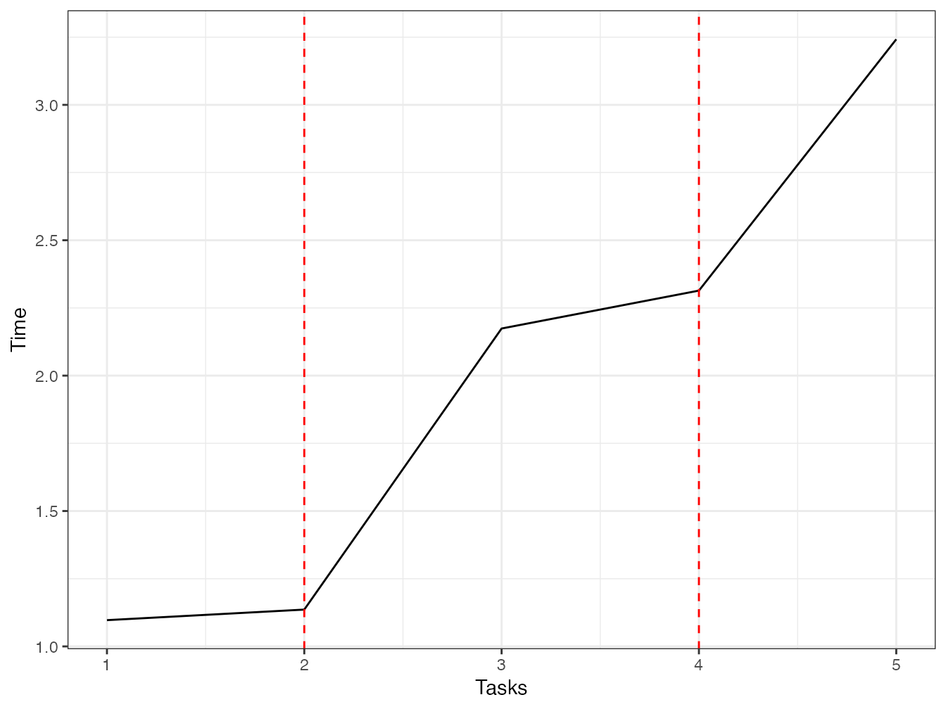

Figure 2.2: Parallel execution time of tasks requiring one second (each task is a one second pause). The number of tasks varies from 1 to twice the number of cores used (equal to 3) plus one.

The theoretical shape of this curve is as follows:

• For a task, the time is equal to one second plus the parallelization setup time.
• The time should remain stable until the number of cores used.
• When all the cores are used (red dotted line), the time should increase by one second and then remain stable until the next limit.

In practice, the computation time is determined by other factors that are difficult to predict. The best practice is to adapt the number of tasks to the number of cores, otherwise performance will be lost.

2.6.2 parLapply (socket)

parLapply requires to create a cluster, export the useful variables on each node, load the necessary packages on each node, execute the code and finally stop the cluster. The code for each step can be found in the mclapply.hack function above.

For everyday use, mclapply is faster, except on Windows, and simpler (including on Windows thanks to the above workaround).

2.6.3 foreach

2.6.3.1 How it works

The foreach package allows advanced use of parallelization. Read its vignettes.

# Manual
vignette("foreach", "foreach")
# Nested loops
vignette("nested", "foreach")

Regardless of parallelization, foreach redefines for loops.

for (i in 1:3) {
    f(i)
}
# becomes
library("foreach")

## 
## Attaching package: 'foreach'

## The following objects are masked from 'package:purrr':
## 
##     accumulate, when

foreach(i = 1:3) %do% {
    f(i)
}

## [[1]]
## [1] 1
## 
## [[2]]
## [1] 2
## 
## [[3]]
## [1] 3

The foreach function returns a list containing the results of each loop. The elements of the list can be combined by any function, such as c.

foreach(i = 1:3, .combine = "c") %do% {
    f(i)
}

## [1] 1 2 3

The foreach function is capable of using iterators, that is, functions that pass to the loop only the data it needs without loading the rest into memory. Here, the icount iterator passes the values 1, 2 and 3 individually, without loading the 1:3 vector into memory.

library("iterators")
foreach(i = icount(3), .combine = "c") %do% {
    f(i)
}

## [1] 1 2 3

It is therefore very useful when each object of the loop uses a large amount of memory.

2.6.3.2 Parallelization

Replacing the %do% operator with %dopar% parallelizes loops, provided that an adapter, i.e. an intermediate package between foreach and a package implementing parallelization, is loaded. doParallel is an adapter for using the parallel package that comes with R.

library(doParallel)
registerDoParallel(cores = nbCores)
# Serial
system.time(foreach(i = icount(nbCores), .combine = "c") %do%
    {
        f(i)
    })

##    user  system elapsed 
##   0.002   0.000   1.031

# Parallel
system.time(foreach(i = icount(nbCores), .combine = "c") %dopar%
    {
        f(i)
    })

##    user  system elapsed 
##   0.009   0.015   0.392

The fixed cost of parallelization is low.

2.6.4 future

The future package is used to abstract the code of the parallelization implementation. It is at the centre of an ecosystem of packages that facilitate its use²⁷.

The parallelization strategy used is declared by the plan() function. The default strategy is sequential, i.e. single-task. The multicore and multisession strategies are based respectively on the fork and socket techniques seen above. Other strategies are available for using physical clusters (several computers prepared to run R together): the future documentation details how to do this.

Here we will use the multisession strategy, which works on the local computer, whatever its operating system.

library("future")
# Socket strategy on all available cores except 1
usedCores <- availableCores() - 1
plan(multisession, workers = usedCores)

The future.apply package allows all *apply() and replicate() loops to be effortlessly parallelized by prefixing their names with future_.

library("future.apply")
system.time(future_replicate(usedCores - 1, f(usedCores)))

##    user  system elapsed 
##   0.066   0.002   0.433

foreach loops can be parallelized with the doFuture package by simply replacing %dopar% with %dofuture%.

library("doFuture")
system.time(foreach(i = icount(nbCores), .combine = "c") %dofuture%
    {
        f(i)
    })

##    user  system elapsed 
##   0.079   0.003   0.562

The strategy is reset to sequential at the end.

plan(sequential)

2.7 Case study

This case study tests the different techniques seen above to solve a concrete problem. The objective is to compute the average distance between two points of a random set of 1000 points in a square window of side 1.

Its expectation is computable²⁸. It is equal to \(\frac{2+\sqrt{2}+5\ln{(1+\sqrt{2})}}{15} \approx 0.5214\).

2.7.1 Creation of the data

The point set is created with the spatstat package.

NbPoints <- 1000
library("spatstat")
X <- runifpoint(NbPoints)

2.7.2 Spatstat

The pairdist() function of spatstat returns the matrix of distances between points. The average distance is calculated by dividing the sum by the number of pairs of distinct points.

mb <- microbenchmark(d <- sum(pairdist(X))/NbPoints/(NbPoints -
    1))
# suppressMessages to eliminate useless messages
suppressMessages(autoplot(mb))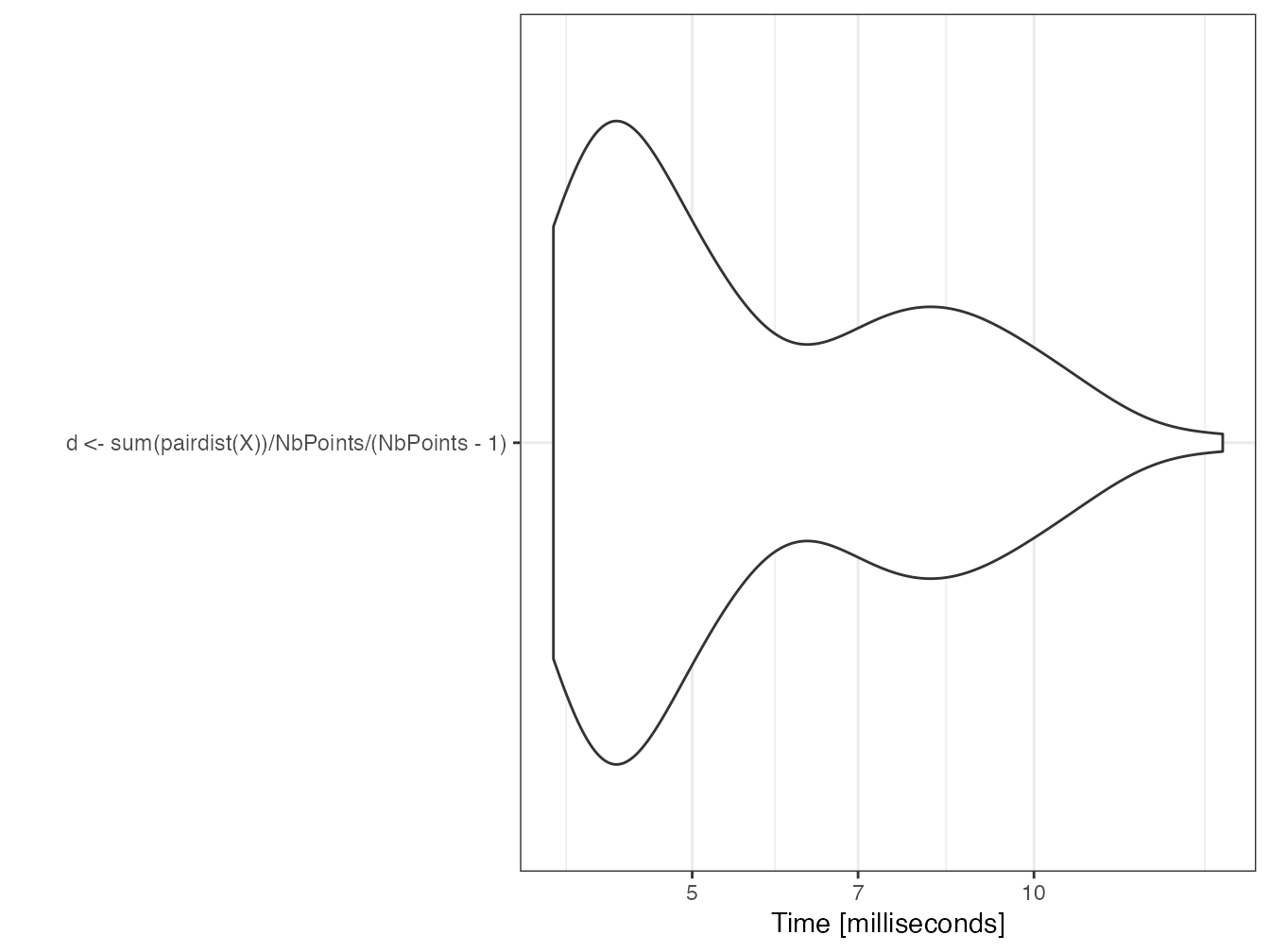

d

## [1] 0.5154879

The function is fast because it is coded in C language in the spatstat package for the core of its calculations.

2.7.3 apply

The distance can be calculated by two nested sapply().

fsapply1 <- function() {
    distances <- sapply(1:NbPoints, function(i) sapply(1:NbPoints,
        function(j) sqrt((X$x[i] - X$x[j])^2 + (X$y[i] - X$y[j])^2)))
    return(sum(distances)/NbPoints/(NbPoints - 1))
}
system.time(d <- fsapply1())

##    user  system elapsed 
##   3.869   0.021   3.900

d

## [1] 0.5154879

Some time can be saved by replacing sapply with vapply: the format of the results does not have to be determined by the function. The gain is negligible on a long computation like this one but important for short computations.

fsapply2 <- function() {
    distances <- vapply(1:NbPoints, function(i) vapply(1:NbPoints,
        function(j) sqrt((X$x[i] - X$x[j])^2 + (X$y[i] - X$y[j])^2),
        0), 1:1000 + 0)
    return(sum(distances)/NbPoints/(NbPoints - 1))
}
system.time(d <- fsapply2())

##    user  system elapsed 
##   3.849   0.010   3.862

d

## [1] 0.5154879

The output format is not always obvious to write:

• it must respect the size of the data: a vector of size 1000 for the outer loop, a scalar for the inner loop.
• it must respect the type: 0 for an integer, 0.0 for a real number. In the outer loop, adding 0.0 to the vector of integers turns it into a vector of real numbers.

A more significant improvement is to compute the square roots only at the end of the loop, to take advantage of the vectorization of the function.

fsapply3 <- function() {
    distances <- vapply(1:NbPoints, function(i) vapply(1:NbPoints,
        function(j) (X$x[i] - X$x[j])^2 + (X$y[i] - X$y[j])^2,
        0), 1:1000 + 0)
    return(sum(sqrt(distances))/NbPoints/(NbPoints - 1))
}
system.time(d <- fsapply3())

##    user  system elapsed 
##   3.800   0.009   3.811

d

## [1] 0.5154879

The computations are performed twice (distance between points \(i\) and \(j\), but also between points \(j\) and \(i\)): a test on the indices allows to divide the time almost by 2 (not quite because the loops without computation, which return \(0\), take time).

fsapply4 <- function() {
    distances <- vapply(1:NbPoints, function(i) {
        vapply(1:NbPoints, function(j) {
            if (j > i) {
                (X$x[i] - X$x[j])^2 + (X$y[i] - X$y[j])^2
            } else {
                0
            }
        }, 0)
    }, 1:1000 + 0)
    return(sum(sqrt(distances))/NbPoints/(NbPoints - 1) * 2)
}
system.time(d <- fsapply4())

##    user  system elapsed 
##   2.232   0.003   2.235

d

## [1] 0.5154879

In parallel, the computation time is not improved on Windows because the individual tasks are too short. On MacOS or Linux, the computation is accelerated.

fsapply5 <- function() {
    distances <- mclapply(1:NbPoints, function(i) {
        vapply(1:NbPoints, function(j) {
            if (j > i) {
                (X$x[i] - X$x[j])^2 + (X$y[i] - X$y[j])^2
            } else {
                0
            }
        }, 0)
    })
    return(sum(sqrt(simplify2array(distances)))/NbPoints/(NbPoints -
        1) * 2)
}
system.time(d <- fsapply5())

##    user  system elapsed 
##   2.422   0.245   1.361

d

## [1] 0.5154879

2.7.4 future.apply

The fsapply4() function optimised above can be parallelled directly by prefixing the vapply function with future_. Only the main loop is parallelized: nesting future_vapply() would collapse performance.

library("future.apply")
# Socket strategy on all available cores except 1
plan(multisession, workers = availableCores() - 1)
future_fsapply4_ <- function() {
    distances <- future_vapply(1:NbPoints, function(i) {
        vapply(1:NbPoints, function(j) {
            if (j > i) {
                (X$x[i] - X$x[j])^2 + (X$y[i] - X$y[j])^2
            } else {
                0
            }
        }, 0)
    }, 1:1000 + 0)
    return(sum(sqrt(distances))/NbPoints/(NbPoints - 1) * 2)
}
system.time(d <- future_fsapply4_())

##    user  system elapsed 
##   0.123   0.013   1.242

d

## [1] 0.5154879

plan(sequential)

2.7.5 for loop

A for loop is faster and consumes less memory because it does not store the distance matrix.

distance <- 0
ffor <- function() {
    for (i in 1:(NbPoints - 1)) {
        for (j in (i + 1):NbPoints) {
            distance <- distance + sqrt((X$x[i] - X$x[j])^2 +
                (X$y[i] - X$y[j])^2)
        }
    }
    return(distance/NbPoints/(NbPoints - 1) * 2)
}
# Calculation time, stored
(for_time <- system.time(d <- ffor()))

##    user  system elapsed 
##   1.398   0.008   1.405

d

## [1] 0.5154879

This is the simplest and most efficient way to write this code with core R and no parallelization.

2.7.6 foreach loop

Parallelization executes for loops inside a foreach loop, which is quite efficient. However, distances are calculated twice.

registerDoParallel(cores = detectCores())
fforeach3 <- function(Y) {
  distances <- foreach(
    i = icount(Y$n), 
    .combine = '+') %dopar% {
      distance <- 0
      for (j in 1:Y$n) {
        distance <- distance + 
          sqrt((Y$x[i] - Y$x[j])^2 + (Y$y[i] - Y$y[j])^2)
      }
      distance
    }
  return(distances / Y$n / (Y$n - 1))
}
system.time(d <- fforeach3(X))

##    user  system elapsed 
##   3.409   0.588   1.152

d

## [1] 0.5154879

It is possible to nest two foreach loops, but they are extremely slow compared with a simple loop. The test is run here with 10 times fewer points, so 100 times fewer distances to calculate.

NbPointsReduit <- 100
Y <- runifpoint(NbPointsReduit)
fforeach1 <- function(Y) {
    distances <- foreach(i = 1:NbPointsReduit, .combine = "cbind") %:%
        foreach(j = 1:NbPointsReduit, .combine = "c") %do% {
        if (j > i) {
            (Y$x[i] - Y$x[j])^2 + (Y$y[i] - Y$y[j])^2
        } else {
            0
        }
    }
    return(sum(sqrt(distances))/NbPointsReduit/(NbPointsReduit -
        1) * 2)
}
system.time(d <- fforeach1(Y))

##    user  system elapsed 
##   1.639   0.014   1.653

d

## [1] 0.5304197

Nested foreach loops should be reserved for very long tasks (several seconds at least) to compensate the fixed costs of setting them up.

2.7.7 RCpp

The C++ function to calculate distances is the following.

#include <Rcpp.h>
using namespace Rcpp;

// [[Rcpp::export]]
double MeanDistance(NumericVector x, NumericVector y) {
  double distance=0;
  double dx, dy;
  for (int i=0; i < (x.length()-1); i++) {
    for (int j=i+1; j < x.length(); j++) {
    // Calculate distance
        dx = x[i]-x[j];
        dy = y[i]-y[j];
        distance += sqrt(dx*dx + dy*dy);
    }
  }
  return distance/(double)(x.length()/2*(x.length()-1));
}

It is called in R very simply. The computation time is very short.

mb <- microbenchmark(d <- MeanDistance(X$x, X$y))
# suppressMessages to eliminate superfluous messages
suppressMessages(autoplot(mb))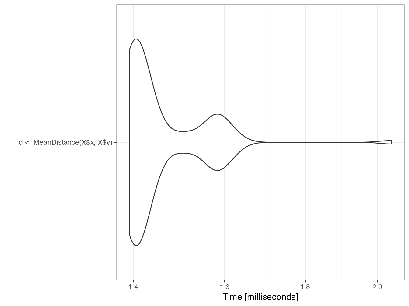

d

## [1] 0.5154879

2.7.8 RcppParallel

RcppParallel allows to interface parallelized C++ code, at the cost of a more complex syntax than RCpp. Documentation is available²⁹.

The C++ function exported to R does not perform the computations but only organizes the parallel execution of another, non-exported, function of type Worker.

Two (C++) parallelization functions are available for two types of tasks:

• parallelReduce to accumulate a value, used here to sum distances.
• parallelFor to fill a result matrix.

The syntax of the Worker is a bit tricky but simple enough to adapt: the constructors initialize the C variables from the values passed by R and declare the parallelization.

// [[Rcpp::depends(RcppParallel)]]
#include <Rcpp.h>
#include <RcppParallel.h>
using namespace Rcpp;
using namespace RcppParallel;

// Working function, not exported
struct TotalDistanceWrkr : public Worker
{
  // source vectors
  const RVector<double> Rx;
  const RVector<double> Ry;
  
  // accumulated value
  double distance;
   
  // constructors
  TotalDistanceWrkr(const NumericVector x, const NumericVector y) :
    Rx(x), Ry(y), distance(0) {}
  TotalDistanceWrkr(const TotalDistanceWrkr& totalDistanceWrkr, Split) :
    Rx(totalDistanceWrkr.Rx), Ry(totalDistanceWrkr.Ry),  distance(0) {}
  
  // count neighbors
  void operator()(std::size_t begin, std::size_t end) {
    double dx, dy;
    unsigned int Npoints = Rx.length();

    for (unsigned int i = begin; i < end; i++) {
      for (unsigned int j=i+1; j < Npoints; j++) {
          // Calculate squared distance
          dx = Rx[i]-Rx[j];
          dy = Ry[i]-Ry[j];
          distance += sqrt(dx*dx + dy*dy);
      }
    }
  }

  // join my value with that of another Sum
  void join(const TotalDistanceWrkr& rhs) { 
    distance += rhs.distance; 
  }
};


// Exported function
// [[Rcpp::export]]
double TotalDistance(NumericVector x, NumericVector y) {
  
  // Declare TotalDistanceWrkr instance
  TotalDistanceWrkr totalDistanceWrkr(x, y);
  
  // call parallel_reduce to start the work
  parallelReduce(0, x.length(), totalDistanceWrkr);
  
  // return the result
  return totalDistanceWrkr.distance;
}

The usage in R is identical to the usage of C++ functions interfaced by RCpp.

(mb <- microbenchmark(d <- TotalDistance(X$x, X$y)/NbPoints/(NbPoints -
    1) * 2))

## Unit: microseconds
##                                                      expr
##  d <- TotalDistance(X$x, X$y)/NbPoints/(NbPoints - 1) * 2
##     min      lq     mean   median       uq      max neval
##  454.71 793.708 821.3327 797.6825 811.2365 1648.278   100

# suppressMessages to eliminate superfluous messages
suppressMessages(autoplot(mb))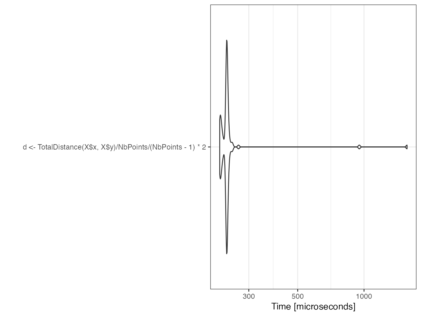

d

## [1] 0.5154879

The setup time for parallel tasks is much longer than the serial computation time.

Multiplying the number of points by 50, the serial computation time must be multiplied by about 2500.

NbPoints <- 50000
X <- runifpoint(NbPoints)
system.time(d <- MeanDistance(X$x, X$y))

##    user  system elapsed 
##   5.199   0.006   5.206

In parallel, the time increases little: parallelization becomes really efficient. This time is to be compared to that of the reference for loop, multiplied by 2500, that is 3512 seconds.

system.time(d <- TotalDistance(X$x, X$y)/NbPoints/(NbPoints -
    1) * 2)

##    user  system elapsed 
##   1.773   0.002   0.444

2.7.9 Conclusions on code speed optimization

From this case study, several lessons can be learned:

• A for loop is a good basis for repetitive calculations, faster than vapply(), simple to read and write.
• foreach loops are extremely effective for parallelizing for loops;
• Optimized functions may exist in R packages for common tasks (here, the pairdist() function of spatstat is two orders of magnitude faster than the for loop).
• the future.apply package makes it very easy to parallelize code that has already been written with *apply() functions, regardless of the hardware used;
• The use of C++ code allows to speed up the calculations significantly, by three orders of magnitude here.
• Parallelization of the C++ code further divides the computation time by about half the number of cores for long computations.

Beyond this example, optimizing computation time in R can be complicated if it involves parallelization and writing C++ code. The effort must therefore be concentrated on the really long computations while the readability of the code must remain the priority for the current code. C code is quite easy to integrate with RCpp and its parallelization is not very expensive with RCppParallel.

The use of for loops is no longer penalized since version 3.5 of R. Writing vector code, using sapply() is still justified for its readability.

The choice of parallelizing the code must be evaluated according to the execution time of each parallelizable task. If it exceeds a few seconds, parallelization is justified.

2.8 Workflow

The targets package allows you to manage a workflow, i.e. to break down the code into elementary tasks called targets that follow each other, the result of which is stored in a variable, itself saved on disk. In case of a change in the code or in the data used, only the targets concerned are reevaluated.

The operation of the flow is similar to that of a cache, but does not depend on the computer on which it runs. It is also possible to integrate the flow into a document project (see section 4.9), and even to use a computing cluster to process the tasks in parallel.

2.8.1 How it works

The documentation³⁰ of targets is detailed and provides a worked example to learn how to use the package³¹. It is not repeated here, but the principles of how the flow works are explained..

The workflow is unique for a given project. It is coded in the _targets.R file at the root of the project. It contains:

• Global commands, such as loading packages.
• A list of targets, which describe the code to be executed and the variable that stores their result.

The workflow is run by the tar_make() function, which updates the targets that need it. Its content is placed in the _targets folder. Stored variables are read by tar_read().

If the project requires long computations, targets can be used to run only those that are necessary. If the project is shared or placed under source control (chapter 3), the result of the computations is also integrated. Finally, if the project is a document (chapter 4), its formatting is completely independent of the calculation of its content, for possibly considerable time saving.

2.8.2 Minimal example

The following example is even simpler than the one in the targets manual, which will allow you to go further. It takes up the previous case study: a set of points is generated and the average distance between the points is calculated. A map of the points is also drawn. Each of these three operations is a target in the vocabulary of targets.

The workflow file is therefore the following:

# File _targets.R 
library("targets")
tar_option_set(packages = c("spatstat", "dbmss"))
list(
  # Draw points
  tar_target(X,
    runifpoint(NbPoints)
  ),
  # Choose Parameters
  tar_target(NbPoints,
    1000
  ),
  # Average Distance
  tar_target(d,
    sum(pairdist(X)) / NbPoints / (NbPoints - 1)
  ),
  # Map
  tar_target(map, 
    autoplot(as.wmppp(X))
  )
)

The global commands consist in loading the targets package itself and then listing the packages needed for the code. The execution of the workflow takes place in a new instance of R.

The targets are then listed. Each one is declared by the tar_target() function whose first argument is the name of the target, which will be the name of the variable that will receive the result. The second argument is the code that produces the result. Targets are very simple here and can be written in a single command. When this is not the case, each target can be written as a function, stored in a separate code file loaded by the source() function at the beginning of the workflow file.

The tar_visnetwork command displays the sequence of targets and their possibly obsolete status.

library("targets")
tar_visnetwork()

The order of declaration of the targets in the list is not important: they are ordered automatically.

The workflow is run by tar_make().

tar_make()

## ▶ dispatched target NbPoints
## ● completed target NbPoints [1.31 seconds]
## ▶ dispatched target X
## ● completed target X [0.002 seconds]
## ▶ dispatched target d
## ● completed target d [0.016 seconds]
## ▶ dispatched target map
## ● completed target map [0.029 seconds]
## ▶ ended pipeline [1.516 seconds]

The workflow is now up to date and tar_make() does not recompute anything.

tar_visnetwork()

tar_make()

## ✔ skipped target NbPoints
## ✔ skipped target X
## ✔ skipped target d
## ✔ skipped target map
## ✔ skipped pipeline [0.081 seconds]

The results are read by tar_read().

tar_read(d)

## [1] 0.5165293

tar_read(map)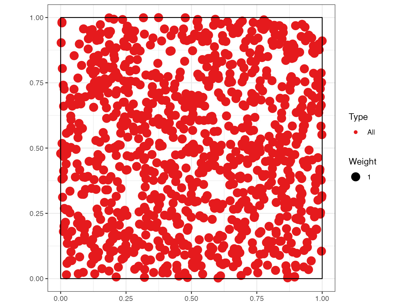

2.8.3 Practical interest

In this example, targets complicates writing the code and tar_make() is much slower than simply executing the code it processes because it has to check if the targets are up to date. In a real project that requires long computations, processing the status of the targets is negligible and the time saved by just evaluating the necessary targets is considerable. The definition of targets remains a constraint, but forces the user to structure their project rigorously.