7 Shiny

Shiny allows to publish an interactive application using R code as a web site. The site can run locally, on a user’s workstation that launches it from RStudio, or online, on a dedicated server running Shiny Server¹¹⁹.

Basically, a form allows to enter the arguments of a function and a visualization window to display the results of the calculation.

A Shiny application makes the execution of the code very simple, even for users not familiar with R, but obviously limits the possibilities.

7.1 First application

In RStudio, create an application with the menu “File > New File > Shiny Web App…”, enter the name of the application “MyShinyApp” and select the folder where to put it.

The name of the application has been used to create a folder that we now need to transform into a project (project menu in the top right of RStudio, “New Project > Existing Directory”, select the application folder).

The application file named app.R contains two functions: ui() which defines the GUI and server() which contains the R code to be executed. The application can be launched by clicking on Run App in the code window.

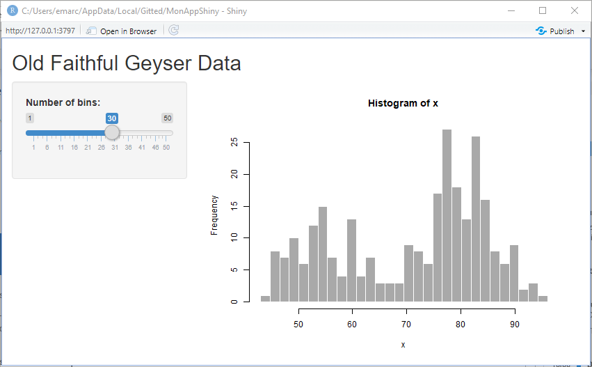
Figure 7.1: Shiny Application Old Faithful Geyser Data.

The correspondence between the displayed window (figure 7.1) and the ui() function code is easy to see:

The title of the application is displayed by the titlePanel() function.
The slider that sets the number of bars in the histogram is created by sliderInput().
The sidebarLayout() function sets the layout of the page elements, sidebarPanel for the input controls and mainPanel() for the result display.

The result is displayed by the plotOutput() function whose argument is the name of an element of output, the variable filled by the server() function.

Any modification of an element of the interface, precisely of an element displayed by a function whose name ends with Input() (there are some for all types of inputs, for example textInput()) of Shiny causes server() to be executed and the elements of output to be updated.

7.2 More elaborate application

7.2.1 Working method

An application is created by choosing:

A window layout.
The controls for entering parameters (intput).
The controls for displaying the results (output).

The code to process the inputs and produce the outputs is then written to server().

The RStudio tutorial¹²⁰ is very detailed and should be used to go further.

7.2.2 Example

This simple application uses the scholar package to query Google Scholar and get the bibliometric data of an author from his or her identifier.

The app.R file contains all the code and is built incrementally here. The full application, with graphical output in addition to its simplified version presented here is available on GitHub¹²¹.

The beginning of the code consists of preparing the application to run by loading the necessary packages:

# Prepare the application ####
# Load packages
library("shiny")
library("tidyverse")

The code of the complete application includes a function to install the missing packages, to be executed only when the application is executed on a workstation (on a server, the management of packages is not the responsibility of the application).

The user interface is as follows:

# UI ####
ui <- fluidPage(
  # Application title
  titlePanel("Bibliometrics"),
  
  sidebarLayout(
    sidebarPanel(
      helpText("Enter the Google Scholar ID of an author."),
      textInput("AuthorID", "Google Scholar ID", "4iLBmbUAAAAJ"),
      # End of input
      br(),
      # Display author's name and h
      uiOutput("name"),
      uiOutput("h")
    ),
    # Show plots in the main panel
    mainPanel(
      plotOutput("network"),
      plotOutput("citations")
    )
  )
)

The application window is fluid, i.e. it reorganizes itself when its size changes, and is composed of a side panel (for text input and display) and a main panel, for displaying graphics.

The elements of the side panel are:

A help text: helpText().
A text input field, textInput(), whose arguments are the name, the displayed text, and the default value (an author ID).
A line break: br().
HTML output controls: uiOutput(), whose single argument is the name.

The main panel contains two graphical output controls, plotOutput() whose argument is also the name.

The code to execute to process the inputs and produce the outputs is in the server() function.

# Server logic ####
server <- function(input, output) {
  # Run the get_profile function only once ####
  # Store the author profile
  AuthorProfile <- reactiveVal()
  # Update it when input$AuthorID is changed
  observeEvent(input$AuthorID, 
               AuthorProfile(get_profile(input$AuthorID)))
  
  # Output ####
  output$name <- renderUI({
    h2(AuthorProfile()$name)
  })
  
  output$h <-
    renderUI({
      a(href = paste0(
        "https://scholar.google.com/citations?user=", 
        input$AuthorID),
        paste("h index:", AuthorProfile()$h_index),
        target = "_blank"
      )
    })
  
  output$citations <- renderPlot({
    get_citation_history(input$AuthorID)  %>%
      ggplot(aes(year, cites)) +
      geom_segment(aes(xend = year, yend = 0),
                   size = 1,
                   color =
                     'darkgrey') +
      geom_point(size = 3, color = 'firebrick') +
      labs(title = "Citations per year",
           caption = "Source: Google Scholar")
  })
  
  output$network <- renderPlot({
    ggplot() + geom_blank()
  })
}

The information needed for the output fields $name and $h (author’s name and h-index) is obtained by the get_profile() function of the scholar package. This function queries the author’s Google Scholar web page and extracts the values from the result: this is a heavy processing, which is better executed only once rather than twice, in the renderUI() functions in charge of computing the values of output$h and output$name.

The simplest code to do this would be as follows:

  # Run the get_profile function only once ####
  # Store the author profile
  AuthorProfile <- get_profile(input$AuthorID)

The difficulty with programming a Shiny application is that any computation referring to an input interface element must be reactive. If the latter code were executed, the following error message would appear: “Operation not allowed without an active reactive context. (You tried to do something that can only be done from inside a reactive expression or observer.)”

In practice, the execution of the code is started by modifying an input control (here: intput$AuthorID). The code referring to one of these controls must be permanently waiting for a modification: it must therefore be placed in particular functions like renderPlot() in the Old Faithful Geyser Data application or renderUI() here. The following code would run without error:

# Output ####
output$name <- renderUI({
    AuthorProfile <- get_profile(input$AuthorID)
    h2(AuthorProfile$name)
})

The call to the value of the input$AuthorID control does occur in a reactive function (but get_profile() would have to be used a second time in the calculation of output$h, which we want to avoid). The function h2(AuthorProfile$name) produces HTML code, a level 2 title paragraph whose value is passed as an argument.

All functions whose names begin with render in the shiny package are reactive, and each is intended to produce a different type of output, for example text (renderText()) or HTML code (renderUI()).

If code is needed to compute variables common to several output controls (output$name and output$h), it must itself be responsive. Two functions are very useful:

observeEvent() watches for changes in an input control and executes code when they occur.
reactiveVal() allows you to define a reactive variable, which will be modified by the observeEvent() code and will in turn cause other reactive functions that use its value to execute.

So the optimal code creates a reactive variable to store the result of the Google Scholar query in:

# Store the author profile
AuthorProfile <- reactiveVal()

The reactive variable is empty at this point. Its use is then that of a function: AuthorProfile(x) assigns it the value x and AuthorProfile(), without arguments, returns its value. The observeEvent() function is triggered when input$AuthorID is modified and executes the code passed as the second argument, in this case the update of AuthorProfile.

# Update it when input$AuthorID is changed
observeEvent(input$AuthorID, AuthorProfile(get_profile(input$AuthorID)))

Finally, the renderUI() functions that provide output control values use the value of AuthorProfile:

# Output ####
output$name <- renderUI({
    h2(AuthorProfile()$name)
})

Note the parentheses in AuthorProfile(), a reactive variable, as opposed to the AuthorProfile$name syntax for a classic variable.

The value of output$h is an internet link, <a href=... in HTML, written by the a() function of the htmltools package used by renderUI().

output$h <- renderUI({
    a(href = paste0("https://scholar.google.com/citations?user=",
        input$AuthorID), paste("h index:", AuthorProfile()$h_index),
        target = "_blank")
})

The link is to the author’s Google Scholar page. The value displayed is its h index. The argument target = "_blank" indicates that the link should be opened in a new browser window.

The output$citations graph is created by the renderPlot() reactive function. The data provided by the get_citation_history() function of scholar (which queries the Google Scholar API) is processed by ggplot().

Finally, the output$network graph is an empty graph in this simplified version of the application.

The full application takes this code and adds error handling in case the author code does not exist on Google Scholar and the co-author network graph.

7.3 Hosting

A Shiny application is not necessarily hosted by a web server: it can be run on users’ workstations if they have R.

For a wider use, a dedicated server is necessary. Shinyapps.io¹²² is a service from RStudio that allows to host 5 Shiny applications for free with a maximum uptime of 5 hours per month.

First of all, you have to open an account on the site, preferably with your GitHub identifiers. To allow the management of online applications directly from RStudio, you must then install the rsconnect package and set it up:

rsconnect::setAccountInfo(name = "prenom.nom", token = "xxx",
    secret = "<SECRET>")

The exact code, along with the username and token to use, are displayed on the Shinyapps.io homepage: click on “Show Secret”, copy the code and paste it into the RStudio console to run it. A “Publish” button is available just to the right of the “Run App” button. Click on it and validate the publication (figure 7.2).

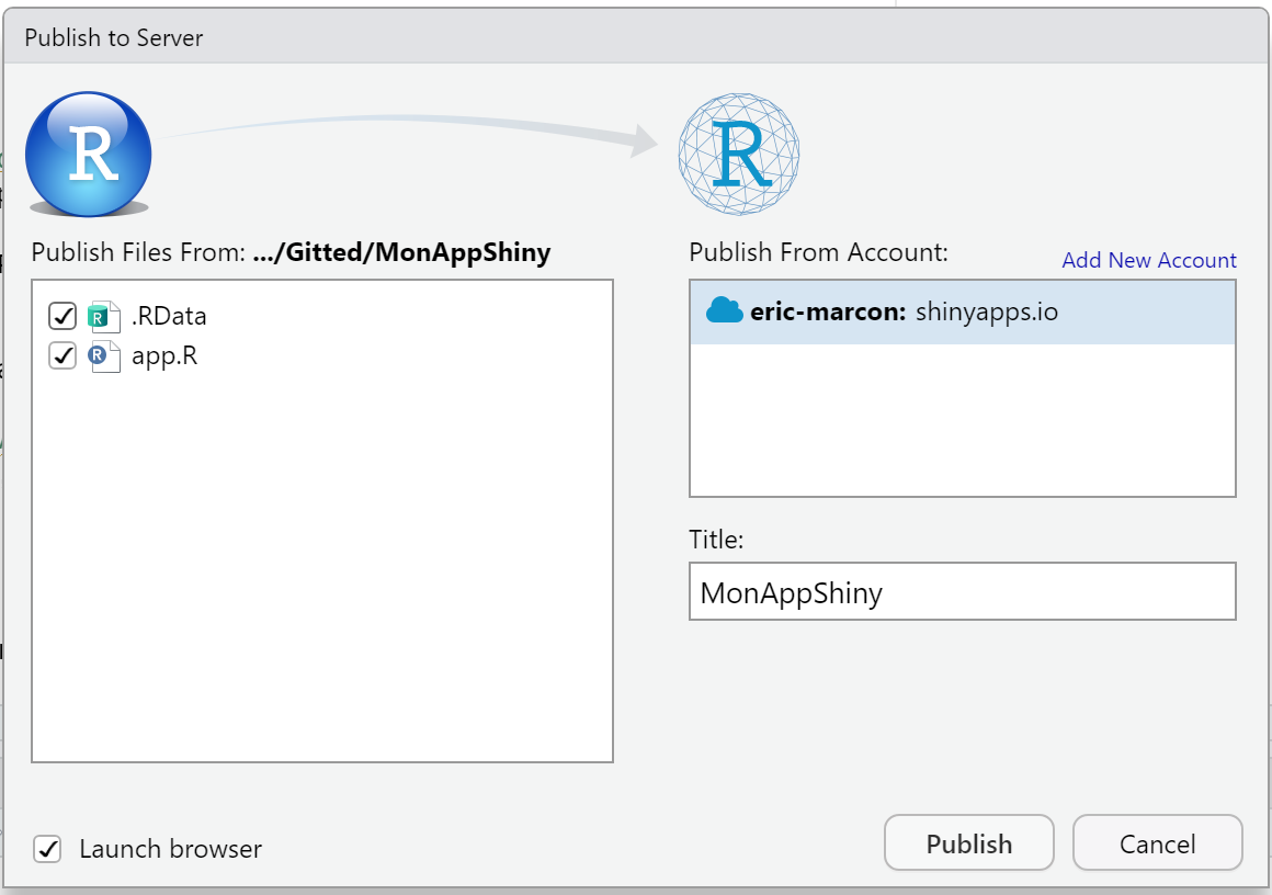
Figure 7.2: Publication of the Shiny application on Shinyapps.io.

The application is now available at https://firstname-lastname.shinyapps.io/MyShinyApp/

The “Bibliometrics” application does not work on Shinyapps.io because the way the Scholar package queries Google Scholar is not supported. Most Shiny applications work without difficulty, as long as they don’t require complex networking features.

6 Continuous integration

8 Teaching with R