Spatial Accumulation of Diversity — accum

A spatial accumulation is a measure of diversity with respect to the distance from individuals.

Usage

# S3 method for class 'accum_sp'
plot(
  x,
  ...,
  q = dimnames(x$accumulation)$q[1],
  type = "l",
  main = "accumulation of ...",
  xlab = "Sample size...",
  ylab = "Diversity...",
  ylim = NULL,
  show_h0 = TRUE,
  line_width = 2,
  col_shade = "grey75",
  col_border = "red"
)

# S3 method for class 'accum_sp'
autoplot(
  object,
  ...,
  q = dimnames(object$accumulation)$q[1],
  main = "Accumulation of ...",
  xlab = "Sample size...",
  ylab = "Diversity...",
  ylim = NULL,
  show_h0 = TRUE,
  col_shade = "grey75",
  col_border = "red"
)

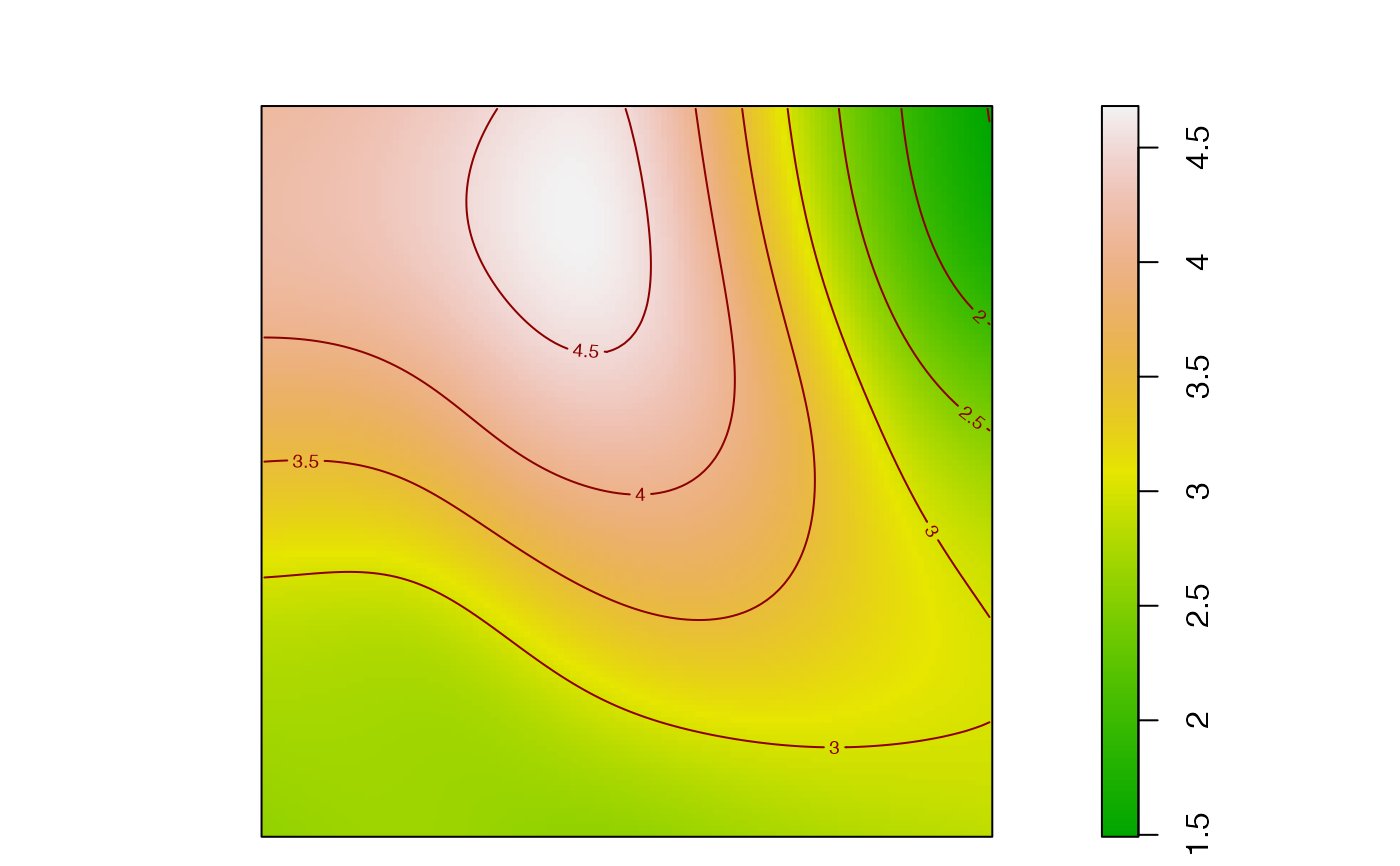
plot_map(
  accum,
  q = dimnames(accum$accumulation)$q[1],
  neighborhood = dplyr::last(colnames(accum$neighborhoods)),
  sigma = spatstat.explore::bw.scott(accum$X, isotropic = TRUE),
  allow_jitter = TRUE,
  weighted = FALSE,
  adjust = 1,
  dim_x = 128,
  dim_y = 128,
  main = "",
  col = grDevices::terrain.colors(256),
  contour = TRUE,
  contour_levels = 10,
  contour_col = "dark red",
  points = FALSE,
  pch = 20,
  point_col = "black",
  suppress_margins = TRUE,
  ...,
  check_arguments = TRUE
)

Arguments

x: an accum_sp object.
...: Additional arguments to be passed to plot, or, in plot_map(), to spatstat.explore::bw.smoothppp and spatstat.explore::density.ppp to control the kernel smoothing and to spatstat.geom::plot.im to plot the image.
q: a number: the order of diversity.
type: plotting parameter. Default is "l".
main: main title of the plot.
xlab: X-axis label.
ylab: Y-axis label.
ylim: limits of the Y-axis, as a vector of two numeric values.
show_h0: if TRUE, the values of the null hypothesis are plotted.
line_width: width of the Diversity Accumulation Curve line.
col_shade: The color of the shaded confidence envelope.
col_border: The color of the borders of the confidence envelope.
object: an accum_sp object.
accum: an object to map.
neighborhood: The neighborhood size, i.e. the number of neighbors or the distance to consider.
sigma: the smoothing bandwidth. The standard deviation of the isotropic smoothing kernel. Either a numerical value, or a function that computes an appropriate value of sigma.
allow_jitter: if TRUE, duplicated points are jittered to avoid their elimination by the smoothing procedure.
weighted: if TRUE, the weight of the points is used by the smoothing procedure.
adjust: force the automatically selected bandwidth to be multiplied by adjust. Setting it to values lower than one (1/2 for example) will sharpen the estimation.
dim_x: the number of columns (pixels) of the resulting map, 128 by default.
dim_y: the number of rows (pixels) of the resulting map, 128 by default.
col: the colors of the map. See spatstat.geom::plot.im for details.
contour: if TRUE, contours are added to the map.
contour_levels: the number of levels of contours.
contour_col: the color of the contour lines.
points: if TRUE, the points that brought the data are added to the map.
pch: the symbol used to represent points.
point_col: the color of the points. Standard base graphic arguments such as main can be used.
suppress_margins: if TRUE, the map has reduced margins.
check_arguments: if TRUE, the function arguments are verified. Should be set to FALSE to save time when the arguments have been checked elsewhere.

Value

plot.accum_sp() returns NULL.

autoplot.accum_sp() returns a ggplot2::ggplot object.

plot_map returns a spatstat.geom::im object that can be used to produce alternative maps.

Details

Objects of class accum_sp contain the value of diversity (accum_sp_diversity objects), entropy (accum_sp_entropy objects) or mixing (accum_sp_mixing objects) at distances from the individuals.

These objects are lists:

X contains the dbmss::wmppp point pattern,
accumulation is a 3-dimensional array, with orders of diveristy in rows, neighborhood size (number of points or distance) in columns and a single slice for the observed entropy, diversity or mixing.
neighborhoods is a similar 3-dimensional array with one slice per point of X.

They can be plotted or mapped.

Examples

# Generate a random community
X <- rspcommunity(1, size = 50, species_number = 10)
# Calculate the species accumulation curve
accum <- accum_sp_hill(X, orders = 0, r = c(0, 0.2), individual = TRUE)
# Plot the local richness at distance = 0.2
plot_map(accum, q = 0, neighborhood = 0.2)