Random communities — rcommunity • divent

Usage

rcommunity(
  n,
  size = sum(abd),
  prob = NULL,
  abd = NULL,
  bootstrap = c("Chao2015", "Marcon2012", "Chao2013"),
  species_number = 300,
  distribution = c("lnorm", "lseries", "geom", "bstick"),
  sd_lnorm = 1,
  prob_geom = 0.1,
  fisher_alpha = 40,
  coverage_estimator = c("ZhangHuang", "Chao", "Turing", "Good"),
  check_arguments = TRUE
)

rspcommunity(
  n,
  size = sum(abd),
  prob = NULL,
  abd = NULL,
  bootstrap = c("Chao2015", "Marcon2012", "Chao2013"),
  species_number = 300,
  distribution = c("lnorm", "lseries", "geom", "bstick"),
  sd_lnorm = 1,
  prob_geom = 0.1,
  fisher_alpha = 40,
  coverage_estimator = c("ZhangHuang", "Chao", "Turing", "Good"),
  spatial = c("Binomial", "Thomas"),
  thomas_scale = 0.2,
  thomas_mu = 10,
  win = spatstat.geom::owin(),
  species_names = NULL,
  weight_distribution = c("Uniform", "Weibull", "Exponential"),
  w_min = 1,
  w_max = 1,
  w_mean = 15,
  weibull_scale = 20,
  weibull_shape = 2,
  check_arguments = TRUE
)

Arguments

n: the number of communities to draw.
size: the number of individuals to draw in each community.
prob: a numeric vector containing probabilities.
abd: a numeric vector containing abundances.
bootstrap: the method used to obtain the probabilities to generate bootstrapped communities from observed abundances. If "Marcon2012", the probabilities are simply the abundances divided by the total number of individuals (Marcon et al. 2012) . If "Chao2013" or "Chao2015" (by default), a more sophisticated approach is used (see as_probabilities) following Chao et al. (2013) or Chao and Jost (2015) .
species_number: the number of species.
distribution: The distribution of species abundances. May be "lnorm" (log-normal), "lseries" (log-series), "geom" (geometric) or "bstick" (broken stick).
sd_lnorm: the simulated log-normal distribution standard deviation. This is the standard deviation on the log scale.
prob_geom: the proportion of resources taken by successive species of the geometric distribution.
fisher_alpha: Fisher's \(\alpha\) in the log-series distribution.
coverage_estimator: an estimator of sample coverage used by coverage.
check_arguments: if TRUE, the function arguments are verified. Should be set to FALSE to save time when the arguments have been checked elsewhere.
spatial: the spatial distribution of points. May be "Binomial" (a completely random point pattern except for its fixed number of points) or "Thomas" for a clustered point pattern with parameters scale and mu.
thomas_scale: in Thomas point patterns, the standard deviation of random displacement (along each coordinate axis) of a point from its cluster center.
thomas_mu: in Thomas point patterns, the mean number of points per cluster. The intensity of the Poisson process of cluster centers is calculated as the number of points (size) per area divided by thomas_mu.
win: the window containing the point pattern. It is an spatstat.geom::owin object. Default is a 1x1 square.
species_names: a vector of characters or of factors containing the possible species names.
weight_distribution: the distribution of point weights. By default, all weight are 1. May be "uniform" for a uniform distribution between w_min and w_max, "weibull" with parameters w_min, weibull_scale and shape or "exponential" with parameter w_mean.
w_min: the minimum weight in a uniform, exponential or Weibull distribution.
w_max: the maximum weight in a uniform distribution.
w_mean: the mean weight in an exponential distribution (i.e. the negative of the inverse of the decay rate).
weibull_scale: the scale parameter in a Weibull distribution.
weibull_shape: the shape parameter in a Weibull distribution.

Value

rcommunity() returns an object of class abundances.

rspcommunity() returns either a spatialized community, which is a dbmss::wmppp object , with PointType values as species names if n=1 or an object of class ppplist (see spatstat.geom::solist) if n>1.

Details

Communities of fixed size are drawn in a multinomial distribution according to the distribution of probabilities provided by prob. An abundance vector abd may be used instead of probabilities, then size is by default the total number of individuals in the vector. Random communities can be built by drawing in a multinomial law following Marcon et al. (2012) , or trying to estimate the distribution of the actual community with probabilities. If bootstrap is "Chao2013", the distribution is estimated by a single parameter model and unobserved species are given equal probabilities. If bootstrap is "Chao2015", a two-parameter model is used and unobserved species follow a geometric distribution.

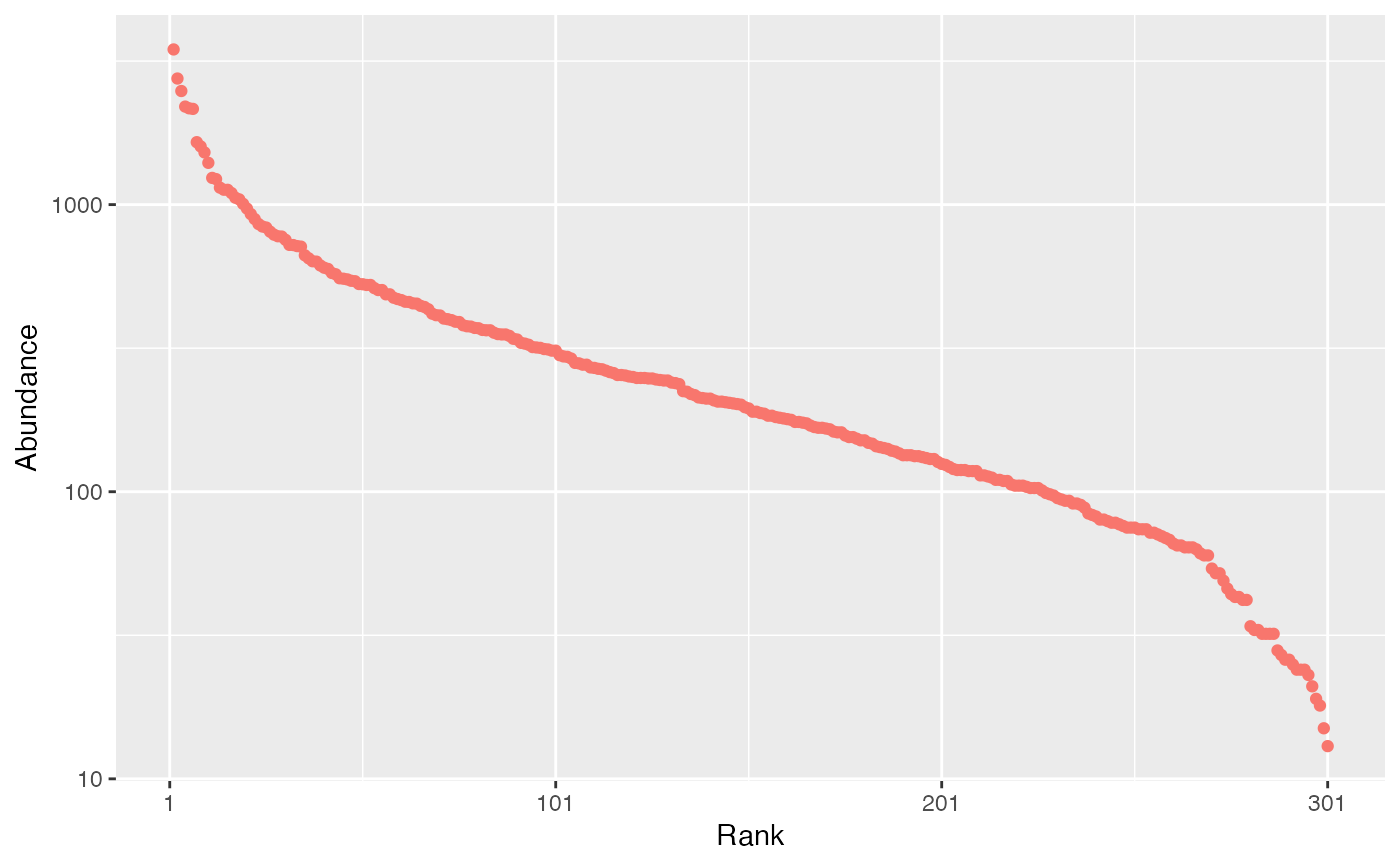
Alternatively, the probabilities may be drawn following a classical distribution: either lognormal ("lnorm") (Preston 1948) with given standard deviation (sd_lnorm; note that the mean is actually a normalizing constant. Its value is set equal to 0 for the simulation of the normal distribution of unnormalized log-abundances), log-series ("lseries") (Fisher et al. 1943) with parameter fisher_alpha, geometric ("geom") (Motomura 1932) with parameter prob_geom, or broken stick ("bstick") (MacArthur 1957) . The number of simulated species is fixed by species_number, except for "lseries" where it is obtained from fisher_alpha and size: \(S = \alpha \ln(1 + size / \alpha)\). Note that the probabilities are drawn once only. If the number of communities to draw, n, is greater than 1, then they are drawn in a multinomial distribution following these probabilities.

Log-normal, log-series and broken-stick distributions are stochastic. The geometric distribution is completely determined by its parameters.

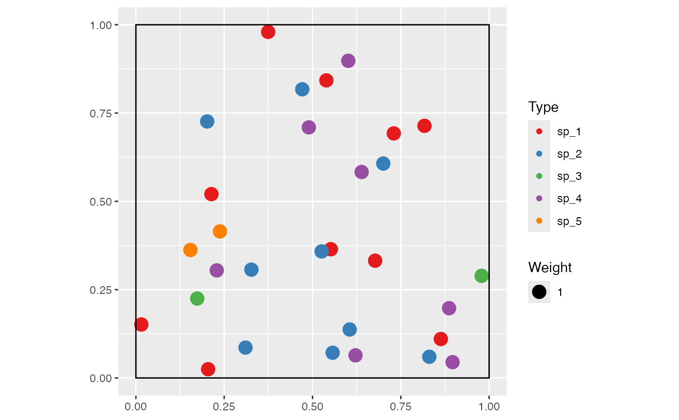
Spatialized communities include the location of individuals in a window, in a dbmss::wmppp object. Several point processes are available, namely binomial (points are uniformly distributed in the window) and Thomas (1949) , which is clustered.

Point weights, that may be for instance the size of the trees in a forest community, can be uniform, follow a Weibull or a negative exponential distribution. The latter describe well the diameter distribution of trees in a forest (Rennolls et al. 1985; Turner 2004) .

References

Chao A, Jost L (2015). “Estimating Diversity and Entropy Profiles via Discovery Rates of New Species.” Methods in Ecology and Evolution, 6(8), 873–882. doi:10.1111/2041-210X.12349 .

Chao A, Wang Y, Jost L (2013). “Entropy and the Species Accumulation Curve: A Novel Entropy Estimator via Discovery Rates of New Species.” Methods in Ecology and Evolution, 4(11), 1091–1100. doi:10.1111/2041-210x.12108 .

Fisher RA, Corbet AS, Williams CB (1943). “The Relation between the Number of Species and the Number of Individuals in a Random Sample of an Animal Population.” Journal of Animal Ecology, 12, 42–58. doi:10.2307/1411 .

MacArthur RH (1957). “On the Relative Abundance of Bird Species.” Proceedings of the National Academy of Sciences of the United States of America, 43(3), 293–295. doi:10.1073/pnas.43.3.293 , 89566.

Marcon E, Hérault B, Baraloto C, Lang G (2012). “The Decomposition of Shannon's Entropy and a Confidence Interval for Beta Diversity.” Oikos, 121(4), 516–522. doi:10.1111/j.1600-0706.2011.19267.x .

Motomura I (1932). “On the statistical treatment of communities.” Zoological Magazine, 44, 379–383.

Preston FW (1948). “The Commonness, and Rarity, of Species.” Ecology, 29(3), 254–283. doi:10.2307/1930989 .

Rennolls K, Geary DN, Rollinson TJD (1985). “Characterizing Diameter Distributions by the Use of the Weibull Distribution.” Forestry, 58(1), 57–66. ISSN 0015-752X, 1464-3626, doi:10.1093/forestry/58.1.57 , 2024-11-07.

Thomas M (1949). “A Generalization of Poisson's Binomial Limit for Use in Ecology.” Biometrika, 36(1/2), 18–25. doi:10.2307/2332526 , 2332526.

Turner IM (2004). The Ecology of Trees in the Tropical Rain Forest, 2nd edition. Cambridge University Press. ISBN 978-0-521-80183-6, doi:10.1017/CBO9780511542206 , 2024-11-07.

Examples

# Generate a community made of 100000 individuals among 300 species and fit it
abundances <- rcommunity(n = 1, size = 1E5,
  species_number = 300, distribution = "lnorm")
autoplot(abundances)

X <- rspcommunity(1, size = 30, species_number = 5)
autoplot(X)