2 Syntax

Deliver the take-home message here.

It can contain several paragraphs.

he main features of Markdown are summarized here. The full documentation is online¹.

2.1 R and other code

R code is included in code chunks:

head(cars)

  speed dist
1     4    2
2     4   10
3     7    4
4     7   22
5     8   16
6     9   10

Similar chunks support other languages such as Python. This template focuses on R but can be used with any other code language supported by Quarto.

2.2 Figures

plot(pressure)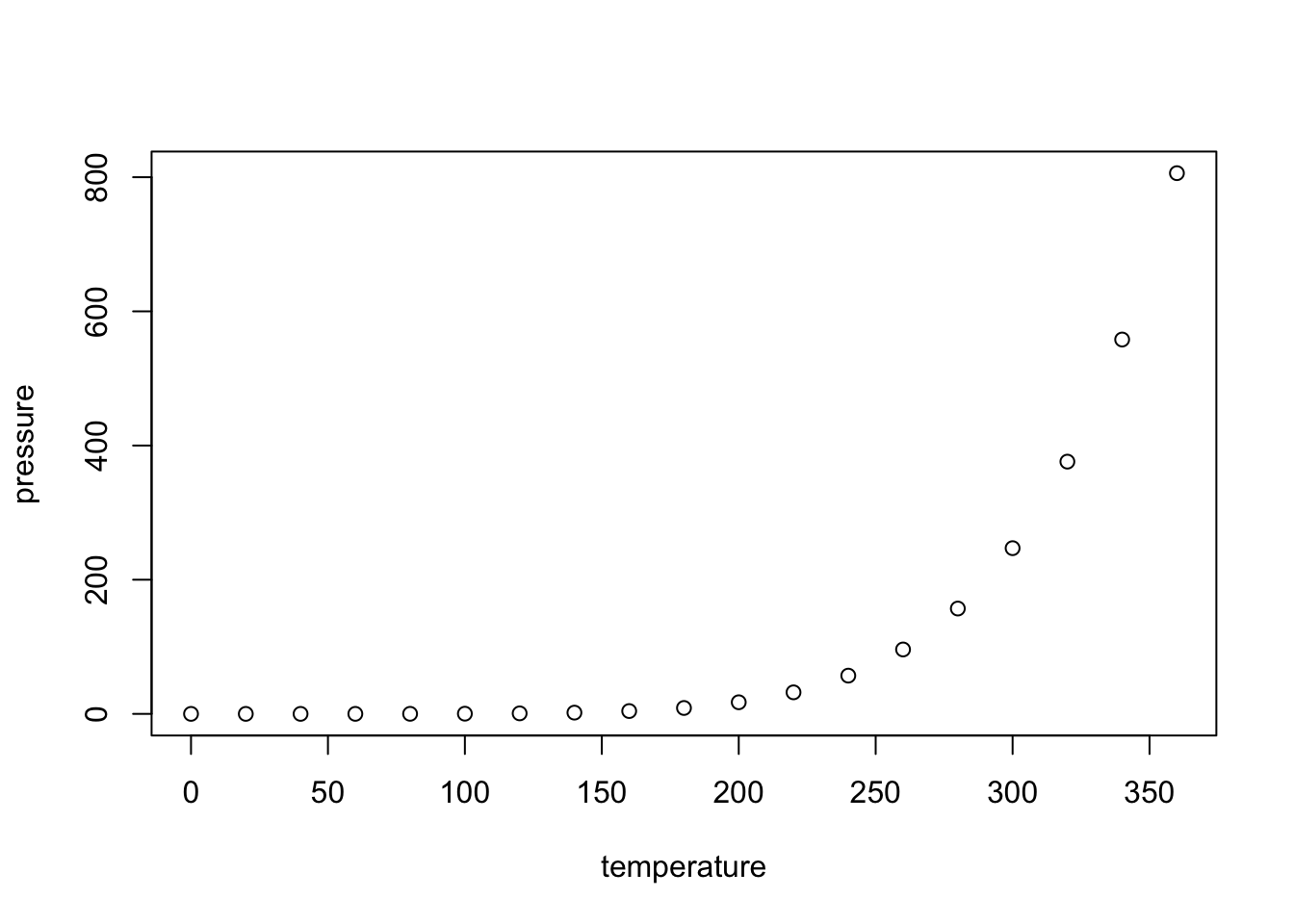

Figure 2.1: Figure *title* with maths : $\pi$ and cross-reference to Table 2.1

Figures can be created by R code (Figure 2.1). A label is associated with each figure: its name is given in the #| label: option of the chunk that produces it. It must start with fig-. Cross-references are made with the command @label, e.g.: @fig-pressure.

Existing figures are integrated into a piece of code by the include_graphics() function, see Figure 2.2.

knitr::include_graphics("images/logo.png")

Figure 2.2: Logo

Systematically place these files in the images folder for the automation of GitHub pages.

2.3 Tables

The horizontal - and vertical separators | allow you to draw a table according to Markdown syntax, but this is not the best method in R.

Tables can also be produced by R code. The content of the table is in a dataframe. The kbl() function prepares the table for display and passes the result to kable_styling() for final formatting.

── Attaching core tidyverse packages ──────────────────────── tidyverse 2.0.0 ──
✔ dplyr     1.1.4     ✔ readr     2.1.5
✔ forcats   1.0.0     ✔ stringr   1.5.1
✔ ggplot2   3.5.2     ✔ tibble    3.2.1
✔ lubridate 1.9.4     ✔ tidyr     1.3.1
✔ purrr     1.0.4     
── Conflicts ────────────────────────────────────────── tidyverse_conflicts() ──
✖ dplyr::filter() masks stats::filter()
✖ dplyr::lag()    masks stats::lag()
ℹ Use the conflicted package (<http://conflicted.r-lib.org/>) to force all conflicts to become errors

Table 2.1: Table created by R, with $\pi$. Dummy legend to demonstrate formatting capacities.

Sepal length	Width	Petal length	Width	Species
5.1	3.5	1.4	0.2	setosa
4.9	3.0	1.4	0.2	setosa
4.7	3.2	1.3	0.2	setosa
4.6	3.1	1.5	0.2	setosa
5.0	3.6	1.4	0.2	setosa
5.4	3.9	1.7	0.4	setosa

The caption is specified by the #| tbl-cap: chunk option.

Always use the booktabs = TRUE argument so that the separator lines are optimal in LaTeX. The bootstrap_options = "striped" option provides more readable tables in HTML.

In LaTeX, longtable = TRUE selects the “longtable” package to format tables. Such tables are placed in the text. Due to limits of the “longtable” package which does not support multi-column layouts, the Stylish Article template uses a workaround that does not allow really long tables to be split into several columns or pages. So, longtable = TRUE only means that the table will be one-column wide and located in the text if possible. If not, it will float.

To use the full width of the page, like Table 2.2, longtable is set to FALSE and table.envir = "table" is added in the arguments of kbl().

Table 2.2: Large table with maths, on two columns

Treatment	Timber	Thinning	Fuelwood	\%AGB lost
Control				0
T1	DBH $\geq$ 50 cm, commercial species, $\approx$ 10 trees/ha			$[12\%-33\%]$
T2	DBH $\geq$ 50 cm, commercial species, $\approx$ 10 trees/ha	DBH $\geq$ 40 cm, non-valuable species, $\approx$ 30 trees/ha		$[33\%-56\%]$
T3	DBH $\geq$ 50 cm, commercial species, $\approx$ 10 trees/ha	DBH $\geq$ 50 cm, non-valuable species, $\approx$ 15 trees/ha	40 cm $\leq$ DBH $\leq$ 50 cm, non-valuable species, $\approx$ 15 trees/ha	$[35\%-56\%]$

This table contains mathematics: the escape = FALSE argument is necessary in kable(). This feature is not yet supported by Quarto in the HTML output.

Finally, the full_width = TRUE argument in kable_styling() adjusts the width of the table to the available width. It must be set for correct formatting of two-column tables in LaTeX.

Note that tables can’t be shown on the first page of the PDF output of the Stylish Article template: they would conflict with the table of contents.

2.4 Lists

Lists are indicated by *, + and - (three hierarchical levels) or numbers 1., i. and A. (numbered lists). Indentation of lists indicates their level: *, + and - may be replaced by - at all levels, but four spaces are needed to nest a list into another.

First element of a list
- sub-list
Second element
Continuation of the list

Leave an empty line before and after the list, but not between its items.

2.5 Math

Equations in LaTeX format can be inserted inline, like $A=\pi r^2$ or isolated like \[e^{i \pi} = -1.\]

They can be numbered, see Equation 2.1, after adding them a label:

\[ A = \pi r^2. \tag{2.1}\]

2.6 Cross-references

Figures and tables have a label declared in their code chunk option tbl.cap or fig.cap, starting with fig- or tbl-.

For equations, the label is added manually by the code {#eq-xxx} after the end of the equation.

Sections can be tagged by ending their title with {#sec-yyy}.

In all cases, the call to the reference is made by @.

2.7 Bibliography

Bibliographic references included in the .bib file declared in the document header can be called by [@CitationKey], in parentheses (Xie, Allaire, and Grolemund 2018), or without square brackets, in the text, as Xie (2016).

The bibliography is processed by Pandoc when producing Word or HTML documents. The bibliographic style can be specified, by adding the line

csl: file_name.csl

in the document header and copying the .csl style file to the project folder. More than a thousand styles are available² and their URL can be used instead of copying the file, e.g.:

csl: https://www.zotero.org/styles/xxx

For PDF documents, the bibliography is managed by natbib. The style is declared in the header:

biblio-style: chicago

It can be changed as long as the appropriate .bst file (by default: chicago.bst) is included in the project.

2.8 Forcing line breaks

Hyphenation is handled automatically in LaTeX. If a word is not hyphenated correctly, add its hyphenation in the preamble of the file with the command hyphenation (words are separated by spaces, hyphenation locations are represented by dashes).

If LaTeX can’t find a solution for the line break, for example because some code is too long a non-breaking block, add the LaTeX command \break to the line break location. Do not leave a space before the command. The HTML document ignores LaTeX commands.

2.9 Languages

Languages are declared in the document header.

The main language of the document (lang) changes the name of some elements, such as the table of contents. The change of language in the document (one of otherlangs) is managed in LaTeX (but not fully in HTML).

For a single word, to ensure correct hyphenation in LaTeX, use the following command, ignored un HTML:

\foreignlanguage{italian}{ciao}

For a paragraph, to also ensure correct quotes and punctuation spacing, use

::: {lang=fr}
"Bonjour" en français!
:::

to obtain:

“Bonjour” en français!

The current language has an effect only in LaTeX output: a space is added before double punctuation in French, the size of spaces is larger at the beginning of sentences in English, etc.

Language codes are used in the header, such as en-US but language names are necessary in LaTeX. Name matches are listed in table 3 of the polyglossia package documentation³. Note that this template uses the “babel” package rather than “polyglossia”.