
Unifying spatially-explicit Rao’s entropy, spatial concentration, and accumulation curves: the different facets of local biodiversity to examine community assembly
Abstract
This chapter introduces a multivariate analytical framework integrating spatial point pattern methodologies and Rao’s entropy to quantify species diversity in ecological communities. Neighbourhood diversity is introduced as a spatialised extension of diversity accumulation curves. Measuring it with Rao’s entropy reveals profound links with Ripley’s K-function, developped to characterise the spatial structure of point patterns. Rao’s neighbourhood entropy can be tested against random labeling and species equivalence null hypotheses to provide insights into ecological processes such as habitat preferences and competitive interactions. The methods are illustrated by applications on simulated datasets and a tropical forest plot in French Guiana. This approach offers a robust means to detect ecological drivers like competition and habitat filtering, enriching our understanding of community assembly while maintaining scalable flexibility across taxonomic, phylogenetic, and functional dimensions.
Keywords
Spatially-explicit diversity, Rao’s entropy, Simpson’s entropy, Species equivalence
1 Introduction
Local biotic and abiotic interactions are recognized as fundamental processes that shape the structure of ecological communities (Keddy 1992; Nemetschek et al. 2025). In particular, the spatial pattern of plant communities may result from the combined effects of seed dispersal, inter-individual (i.e. intra- and inter-specific) competition/facilitation, interactions with natural enemies, and habitat preferences (Dale 1999). The diversity of these abiotic and biotic interactions in space and/or time is a key feature for community assembly and the maintenance of biological diversity (Clark et al. 2010; Cadotte et al. 2012). Consequently, the ecological literature reveals increasing efforts to integrate approaches from phylogenetics, functional and community ecology (Mouquet et al. 2012), to account for the key components of species interactions with their biotic and abiotic environments. Several novel analytical methods incorporating measures of between-species phylogenetic relatedness or functional trait dissimilarities as a surrogate for ecological differences have been developed (Pavoine and Bonsall 2011). Among these methods, some are specifically designed to explicitly account for space (e.g. Pavoine et al. 2011).
The interest of considering local diversity rather than at the scale of the whole community or sampling window has emerged in the literature since Batty (1974). A review can be found in Altieri et al. (2021), with diverse approaches. It is not discussed that the functioning of a community is influenced by its constituent biodiversity, but it is straightforward to consider that each individual is concerned by the diversity of its neighbourhood rather that of the whole community (e.g., Hubbell et al. 2001 showed that tree mortality increased with neighbourhood species richness in a tropical evergreen forest). When mapped data are concerned, such as for instance those on tropical trees provided by large permanent forest plots (Losos and Leigh 2004), the well-developed framework of the spatial point pattern analysis (Ripley 1976, 1977) offers an efficient means of studying the continuous spatial variation in species diversity (Condit et al. 2000; Shimatani 2001a; Rajala and Illian 2012). A synthesis of the opportunities brought by this approach can be found in Wiegand et al. (2017).
Shen et al. (2013) and Pélissier and Goreaud (2015) concomitantly introduced, within the framework of the spatial point pattern analysis, a multitype correlation function that provides a distance-dependent measure of species diversity accounting for non-uniform species differences. Since both contributions independently arrived to very similar approaches, we believe further clarifications are needed to help ecologists to take full advantage of this development. In particular, it is important to relate non-uniform differences to well-known functions of spatial point pattern analysis, namely Ripley’s K-function (Ripley 1977) and its intertype extension, the Kp,q-function (Lotwick and Silverman 1982) on the one hand, and Rao’s quadratic entropy on the other hand (Rao 1982).
The aim of this chapter is thus to introduce the rationale behind the functions of multivariate point pattern analysis that integrate between-species differences in a distance–dependent measure of diversity. It can basically be seen as an extension of the work of Shimatani (2001a) based on Simpson’s entropy to Rao’s entropy, one of the most powerful and flexible measure of species diversity (Pavoine 2012). It is also a particular implementation of the measurement of neighbourhood diversity which possesses some specific features due to the quadratic form of Rao’s entropy. The methods section hereafter makes the synthesis between these originally independent developments and outlines the central role of Rao’s entropy to reconcile them. We finally provide worked examples based on simulated data and on a real dataset from an experimental tropical forest plot in French Guiana.
2 Methods
2.1 From aspatial to spatial diversity
Simpson’s and Rao’s entropies
Simpson’s index of species diversity (Simpson 1949) gives the probability that a randomly selected pair of individuals in a sample is comprised of two different species. It is more than an index: it is a measure of entropy (Jost 2006) and thus should be named Simpson’s entropy. It is estimated with no bias by:
\[\hat{D} = 1 - \sum_{p=1}^S{\frac{n_p \left(n_p - 1 \right)}{n \left(n - 1 \right)}} \tag{1}\]
where \(n\) and \(S\) are the total numbers of individuals and species in the sample, respectively, and \(n_p\) the number of individuals of species \(p\).
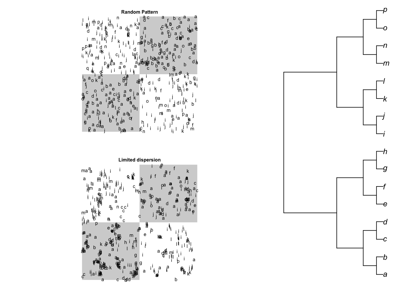
Non-uniform divergences between species allow defining phylogenetic or functional diversity (Pielou 1975). We will note \(d_{p,q}\) the measure of the pairwise divergence between species \(p\) and \(q\). \(d_{p,q} = d_{q,p}\) and \(d_{p,p} = 0\), but the triangular inequality \(d_{p,q} + d_{q,r} \geq d_{p,r}\) that defines a distance is not required. Functional diversity applies to species whose divergences is described by a matrix of dissimilarities, generally built from trait values: see the Paracou example in the Application section below. Phylogenetic diversity applies to species whose phylogeny is described by a tree (an example is in Figure 1) relating them to their ancestors. The divergences between pairs of species, i.e. the height of their first common ancestor in the tree are named cophenetic distances. They are Euclidean. If all tips of the tree (the species) are at the same level, then the cophenetic distances are ultrametric.
Rao’s entropy is the expected divergence between individuals of a randomly selected pair in a sample (Rao 1982). An unbiased estimator (Shimatani 2001b) is:
\[\hat{H}_D = \sum_{p=1}^S\sum_{q=1}^S{\frac{n_p n_q}{n \left(n - 1 \right)}d_{p,q}} \tag{2}\]
\(H_D\) is a measure of diversity commonly used in ecology, namely because it can be linked to ordination methods (Pavoine et al. 2004; Pavoine and Bonsall 2011) when \(d_{p,q}\) are distances.
Taking \(d_{p,q} = 1\) for all \(p \neq q\) and 0 otherwise, \(H_D\) reduces to Simpson’s \(D\) above.
Diversity is scale-dependent: its value increases with the sample size so it needs to be standardized. A common practice consists of estimating the asymptotic diversity, i.e. the diversity of a hypothetical community the available data is assumed to be a representative sample of. For instance, species asymptotic richness is often estimated with the well-known Chao1 estimator (Chao 1984)
The estimators above (Equation 1 and Equation 2) are doubly unbiased: in a finite sample, they estimate entropy taking into account sampling without replacement (Simpson 1949), and they estimate asymptotic diversity assuming sampling with replacement in a large community (Lande 1996).
Diversity accumulation curves
The Species Accumulation Curve (SAC) describes the expectation of the number of observed species with respect to the sample size (Gotelli and Colwell 2001), assuming uniform and independent sampling of individuals or, equivalently, that continuous sampling happens in a community where all species are distributed independently according to homogeneous Poisson point patterns. It can be derived from the distribution of species abundances of the full sample (Ugland et al. 2003). The sample size consists of a number of individuals that can be converted to a sample area assuming the density of individuals is constant. SACs allow to define biodiversity at a given spatial scale. It is an alternative to estimating asymptotic diversity.
Diversity Accumulation Curves (DACs) extend this approach to all measures of diversity. Simpson’s entropy accumulation curves were derived by Chao et al. (2014) and extended straightforwardly to Rao’s entropy applied to ultrametric distances (Marcon and Hérault 2015). Entropy is generally converted into Hill numbers (Jost 2006), but this is not necessary here because the value of entropy can be interpreted. Yet, DACs are aspatial (Rajala and Illian 2012), as they are designed to ignore the spatial pattern of the data. Spatial structure is generally considered as an empirical issue (Gotelli and Colwell 2001), which can be solved laboriously by deriving accumulation curves that take into account the spatial pattern of each species (Picard et al. 2004).
Neighbourhood diversity
Considering biodiversity from the perspective of each individual, whose functioning is assumed to be related to it, requires estimating diversity in its neighbourhood, as argued by Rajala and Illian (2012).
Rather than aspatial diversity accumulation curves, neighbourhood diversity curves can be estimated empirically based on a fully-mapped dataset. The definition of neighbourhood is restricted here to a disc defined by radius \(r\) around each individual. Each of these discs can be considered as a local community whose entropy (e.g. Simpson’s or Rao’s entropy) can be estimated and averaged across sampled individuals (Marcon et al. 2014) to obtain a value of \(\alpha\) entropy, that estimates the expected entropy in the neighbourhood of a random individual. We’ll denote Simpson’s and Rao’s neighbourhood entropies \(D(r)\) and \(H_D(r)\) respectively.
Neighbourhood diversity can be computed with the divent package (Marcon and Puech 2026) for R (R Core Team 2026). The computational burden is heavy for a community of a few thousand individuals because entropy must be estimated around each individual and for each neighbourhood size, with edge-effect corrections: the diversity partially observed in neighbourhoods that do not fit in the sampling window must be extrapolated. An alternative approach, based on spatial statistics, allows the rapid estimation of neighbourhood Simpson’s and Rao’s entropy, and reveals profound connections with the point-process theory.
2.2 Distance-dependent entropy based on the point-process theory
Ripley’s K
The framework of spatial point pattern analysis, as introduced by Ripley (1977), relies on the K-function, defined so that \(\lambda K(r)\) is the expected number of neighbours located within a distance \(r\) of an arbitrary point of the pattern with intensity \(\lambda\). Its classical unbiased estimator for a point pattern located within a finite sampling window is:
\[\hat{K}\left( r \right) = \frac{1}{\hat{\lambda}n} \sum_{i=1}^{n}{\sum_{j=1}^{n}{ \mathbf{1}\left( \|x_i - x_j\| \leq r \right) c\left(i, j, r \right) }} \tag{3}\]
where \(n\) is the number of points of the pattern, \(\lambda\) is the pattern intensity estimated as \(n/A\), with \(A\) the sampling window area. The indicator function \(\mathbf{1}( \|x_i - x_j\| \leq r)\) equals 1 when points \(i\) and \(j\) are less than \(r\) apart, 0 else. \(c(i, j, r)\) is the correction of edge effects equal to 1 when the circle of radius \(r\) fits into the sampling window. When it does not, the isotropic correction proposed by Ripley (1977) applies to windows of any shape thanks to appropriate geometrical considerations (Goreaud and Pélissier 1999) to estimate the number of neighbours with no bias.
The L-function (Besag 1977) modifies the K-function so that its expectation is 0 rather than \(\pi r^2\) if the point process is homogeneous Poisson (i.e. the points are distributed uniformly and independently): \(L(r) = \sqrt{K(r) / \pi} - r\).
A common extension of this univariate function is the intertype (or bivariate) function proposed by Lotwick and Silverman (1982) for marked point patterns, that we will denote \(K_{p,q}\). Here, the mark of a point, called its type, is the species of the individual represented by the point.
\[\hat{K}_{p,q}\left( r \right) = \frac{A}{\hat{\lambda_p}\hat{\lambda_q}} \sum_{i=1}^{n_p}{\sum_{j=1}^{n_q}{ \mathbf{1}\left( \|x_i - x_j\| \leq r \right) c\left(i, j, r \right) }} \tag{4}\]
where \(n_p\) and \(n_q\) are the number of points of types \(p\) and \(q\) respectively. \(\hat{\lambda}_p\) and \(\hat{\lambda}_q\) are their intensities.
\(K(r)\) is a multiscale function of second-order neighbourhood properties of a point pattern, which allows robust tests of statistical significance against the null hypothesis of a random distribution of the points within the sampling window. In contrast, \(K_{p,q}(r)\) allows characterizing the spatial interaction between the two types of points, which can be tested against various null hypotheses. The most interesting ones are the random labelling hypothesis, which means that, conditionally to the point locations, types \(p\) and \(q\) are randomly distributed among points of the pattern, and the population independence hypothesis, meaning that, conditionally to the species-specific spatial patterns, population of type-\(p\) points is independent from population of type-\(q\) points (Goreaud and Pélissier 2003).
A distance-dependent Simpson’s entropy
Shimatani (2001a) derived an estimator of the neighbourhood Simpson’s entropy, \(D(r)\), based on Ripley’s K-function:
\[\hat{D}\left( r \right) = 1 - \sum_{p=1}^S{\frac {\hat{\lambda}_p^2 \hat{K}_p\left( r \right)} {\hat{\lambda}^2 \hat{K}\left( r \right)} } \tag{5}\]
where \(\hat{K}(r)\) and \(\hat{K}_p(r)\) are Ripley’s K-functions for all points of the pattern (no distinction of species) and for points of species \(p\), respectively, with \(\hat{\lambda}\) and \(\hat{\lambda}_p\) the corresponding intensity estimators.
We can define \(K_S(r)\) as a version of \(D(r)\) standardized by \(D\), estimated as:
\[\hat{K}_S\left( r \right) = \hat{D}\left( r \right) / \hat{D} \tag{6}\]
\(D(r)\) tends to \(D\) when \(r\) increases so \(K_S(r)\) tends to 1. It is noticeable that \(K_S(r)\) has an expectation of 1 for any \(r\) under the random labelling hypothesis, i.e. a random distribution of the species names conditionally to the overall spatial pattern (Eckel et al. 2008).
Using the unbiased estimator of \(\hat{K}(r)\), introduced in Equation 3, allows correcting for edge effects in sampling windows of any shape.
In line with Shimatani (2001a), eq. 9, we notice for the following that \(\hat{K}_S(r)\) can also be estimated by considering the pairs of heterospecifics. Equation 5 can be rearranged considering that \(\hat{\lambda}^2 \hat{K}(r) = \sum_p\sum_q{\hat{\lambda}_p \hat{\lambda}_q \hat{K}_{p,q}(r)}\) and \(\sum_p \sum_{q \neq p} {\hat{\lambda}_p \hat{\lambda}_q \hat{K}_{p,q}(r)} = \sum_p \sum_q {\hat{\lambda}_p \hat{\lambda}_q \hat{K}_{p,q}(r)} - \sum_p{\hat{\lambda}_p^2 \hat{K}_p(r)}\). Then it comes from Equation 6 that:
\[\hat{K}_S(r) = \left[ \sum_{p=1}^S{\sum_{q=1, p \ne q}^S {\frac {\hat{\lambda}_p \hat{\lambda}_q \hat{K}_{p,q}\left( r \right)} {\hat{\lambda}^2 \hat{K}\left( r \right)}} } \right] / \hat{D} \tag{7}\]
A generalization to Rao’s entropy
We therefore straightforwardly propose to generalize \(K_S(r)\) introduced above to a normalized, distance-dependent Rao’s quadratic entropy \(K_R(r)\) that integrates Ripley’s correction of edge effects estimated by:
\[\begin{aligned} \hat{K}_R\left( r \right) &= \hat{H}_D\left( r \right) / \hat{H}_D \\ &= \left[ \sum_{p=1}^S{\sum_{q=1, p \ne q}^S{ \frac {\hat{\lambda}_p \hat{\lambda}_q \hat{K}_{p,q}\left( r \right) d_{p,q}} {\hat{\lambda}^2 \hat{K}\left( r \right)}} } \right] / \hat{H}_D \end{aligned} \tag{8}\]
This function has an expectation of 1 under the random labelling hypothesis and gives the mean proportion of Rao’s sample diversity in a disc of radius \(r\) centred on an arbitrary point of the pattern. \(\hat{K}_R(r)\) reduces to \(\hat{K}_S(r)\) when \(d_{p,q} = 1\) for all species \(p \neq q\).
Multitype correlation and \(\beta\) diversity
Whittaker (1960) introduced the framework of diversity partitioning and defined the concepts of \(\alpha\) and \(\beta\) diversity we recall here for the clarity of what follows. \(\alpha\) diversity is the average diversity of continuous areas, such as forest plots or, here, the discs around points that define neighbourhood diversity. In contrast, \(\beta\) diversity characterises how dissimilar discontinuous areas are from each other, defining differentiation \(\beta\) diversity, or from their assemblage, defining proportional \(\beta\) diversity (Jurasinski et al. 2009). \(\gamma\) diversity is in turn the diversity of the assemblage: it can be partitioned into \(\alpha\) and proportional \(\beta\) diversities (Pavoine et al. 2004; Jost 2007).
Our KR- and KS-functions are cumulative functions as is the original K-function of Ripley (1977). This means that they are estimated for a series of concentric neighbourhood discs of increasing radii: they measure their \(\alpha\) diversity with \(D(r)\) and \(H_D(r)\) and standardize it by \(D\) and \(H_D\) respectively. Some authors however prefer to refer to the framework of the pair-correlation function, \(g(r)\) (Stoyan et al. 1987; Wiegand and Moloney 2004), that is the derivative of \(K(r)\), giving the probability to encounter neighbouring points in concentric annuli between \(r\) and \(r + dr\), and relate it to \(\beta\) diversity.
Precisely (Ripley 1977):
\[ g\left( r \right) = \lambda^2 \frac{dK}{2 \pi r dr} \]
Chave and Leigh (2002) defined the \(F(r)\) function as the probability for two individuals located \(r\) apart to belong to the same species. Shen et al. (2013) named \(1 - F(r)\) the “spatially explicit Simpson’s \(\beta\) index of diversity”, denoted \(\beta(r)\) by Shimatani (2001a), that is the probability for two individuals located \(r\) apart to belong different species. We will rather write \(\beta_S(r)\) for consistency with our notation system.
Let \(P(r)\) the probability to find two points in two infinitesimal areas \(dx\) and \(dy\) at distance \(r\) from each other. \(P_p(r)\) is defined the same way for points of species \(p\). Shimatani (2001a) derived \(\beta_S(r)\) as follows, from the relation between \(P(r)\) and \(g(r)\): \(P(r) = \lambda^2 g(r) dx dy\). Assuming two points are \(r\) apart, one at the centre of the disc and one in the annulus between \(r\) and \(r + dr\), their conditional probability to belong to different species is:
\[ \begin{aligned} \beta_S(r) &= 1 - \sum_{p=1}^S{\frac{P_p(r)}{P(r)}} \\ &= 1 - \sum_{p=1}^S{\frac {\lambda^2_p g_p\left( r \right)} {\lambda^2 g\left( r \right)}} \end{aligned} \]
\(\beta_S(r)\) can be straightforwardly generalized to \(\beta_R(r)\), the average divergence between to individuals taken at distance \(r\) (noted \(K_d(r)\) by Shen et al. 2013). The spatially explicit Rao’s \(\beta\) index of diversity is:
\[\beta_R\left( r \right) = \sum_{p=1}^S{\sum_{q=1, p \ne q}^S{\frac {\lambda_p \lambda_q g_{p,q}\left( r \right) d_{p,q}} {\lambda^2 g\left( r \right)}} } \tag{9}\]
where \(g_{p,q} = \lambda_p \lambda_q \frac{dK_{p,q}}{2 \pi r dr}\) is the bivariate g-function.
These measures are actually differentiation \(\beta\) diversity measures sensu Jurasinski et al. (2009): they characterize how different spatial units \(r\) apart are in terms of species composition.
The framework of entropy partitioning (Jost 2007; Marcon et al. 2014) requires \(\beta\) entropy to be the difference between \(\gamma\) entropy (that of neighbourhoods of radius \(r + dr\)) and \(\alpha\) entropy (that of neighbourhoods of radius \(r\)), i.e. \(\beta\) entropy needs to be the derivative of \(H_D(r)\). Yet, although both the numerator and the denominator of \(\beta_R(r)\) are the derivatives of the numerator and the denominator of \(H_D(r)\) (see Equation 8), \(\beta_R(r)\) is not the derivative of \(H_D(r)\). In other words, \(\beta_R(r)\) does not comply with the definition of proportional \(\beta\) diversity. To do that, it should quantify the dissimilarity between the annulii between \(r\) and \(r + dr\) and the discs of radius \(r\), not the infinitesimal areas around their centres.
For this reason, we argue in favour of the cumulative approach, i.e. that of \(\alpha\) diversity (with the KS- and KR-functions), and also because the effect of neighbourhood diversity on the functioning of individuals is more naturally modelled as cumulative.
We do not provide the estimators of \(\beta_S(r)\) and \(\beta_R(r)\) here: they can be found in Shimatani (2001a) and Shen et al. (2013).
2.3 Testing ecological models
The KR-function allows computing phylogenetic or functional entropy in the neighbourhood of individuals with respect to distance. Beyond measuring diversity, it also allows inferring ecological processes responsible of the observed patterns by testing them against appropriate null hypotheses.
The random labelling null hypothesis
The null hypothesis of random labelling originally proposed by Shimatani (2001a) provides a test of departure of \(\hat{K}_R(r)\) from a random distribution of the mark labels among points of the pattern. It allows testing for an absence of interaction between neighbouring points, conditionally to the overall pattern of point locations, so that the probability to find a pair of identical marks is independent of distance. When the function is above 1, the mean diversity within a disc of radius \(r\) from an arbitrary point of the pattern is higher than the total sample diversity, and conversely. Local confidence limits of the random labelling hypothesis at a given significance level can be built from Monte Carlo rank tests (Diggle 1979). This hypothesis basically relies on the assumption that the marks result from a random process that affects individuals a posteriori with regards to the process of point location, so that we have for all \(p\) types of marks \(K_p(r) = K(r)\) (Goreaud and Pélissier 2003; Eckel et al. 2008) and hence \(K_R(r) = 1\). This could for instance corresponds to a multitype process resulting from a disease attack in a plant population that would mark the individuals as sick, non-infected or healthy carriers (see also Eckel et al. 2008 for an example in socio-economics). In the context of species diversity, the random labelling hypothesis corresponds to the absence of any spatial structure, resulting from a process where the species identities would not interfere.
The population independence null hypothesis
A more meaningful hypothesis for species diversity studies is the one of mutually independent populations, postulating that the spatial pattern of each population (i.e., the individuals of the same type) is the realization of a specific spatial process (for instance of limited dispersion) and that the location of points of each population is independent from the location of the points of the other populations in the resulting multivariate pattern. This is a generalization of the population independence hypothesis proposed for testing the bivariate \(K_{p,q}\)-function by Lotwick and Silverman (1982) for which we expect that \(K_{p,q}(r) = \pi r^2\) for any mark \(p \neq q\) (Eckel et al. 2008), and hence, here also, \(K_R(r) = 1\). Note that this hypothesis differs from the random labelling hypothesis, except when all specific spatial patterns result from a stationary Poisson point process (Diggle 1983).
A classical method for testing the mutually independent population hypothesis is to build a Monte Carlo rank test keeping the pattern of each population unchanged but randomizing their relative positions by a random shifting procedure of each pattern around a torus (Goreaud and Pélissier 2003). Such a procedure is cumbersome for highly multivariate patterns and is considered suboptimal for testing diversity patterns.
The species equivalence null hypothesis
More interestingly, \(K_R(r)\) provides opportunities for testing a highly relevant ecological hypothesis for diversity studies, based on \(d_{p,q}\), which quantifies how species differ one from each other. Shuffling between-species distances many times means eliminating their differences and therefore testing a null hypothesis of species equivalence. This null hypothesis can be tested conditionally to the pattern of point locations and to the spatial distribution of the species labels by permuting simultaneously the rows and columns in \(d_{p,q}\), which is equivalent, in the case of a cophenetic distance matrix, to permuting the tips of a hierarchical (taxonomic or phylogenetic) tree (Hardy 2008). It is noteworthy that under the null hypothesis of species equivalence, \(K_S(r)\) provides a theoretical expectation of \(K_R(r)\), i.e. the value expected when \(d_{p,q}\) consists of a uniform between-species distance matrix. When focusing on the species equivalence hypothesis, \(K_R(r) / K_S(r)\), the standardization proposed by Shen et al. (2013), provides a constant expectation of 1 at all distances. With reference to these authors and to the usual notation in point pattern analysis, \(K_R(r) / K_S(r)\) is appropriately designated as \(K_d(r)\).
3 Application
3.1 Simulated data
We provide here a few examples to illustrate how the \(K_R\)-function behaves. All the functions introduced above along with resources for computing tests of statistical significance based on Monte Carlo simulations have been implemented within the ads package (Pélissier and Goreaud 2015). Figures were produced by the dbmss package (Marcon et al. 2015).
We want to test the detection of two major mechanisms responsible for species coexistence. Habitat preference implies that the neighbourhood of a tree, whose abiotic conditions (soil, microclimate) are assumed to be quite homogeneous because of its small spatial extent, is occupied by similar trees, i.e. whose phylogenetic (Webb et al. 2002) or functional dissimilarity (Cornwell et al. 2006) is small, because their preferences are similar. Then, the neighbourhood diversity should be smaller than under the species equivalence null hypothesis. On the other hand, competition for the same resources limits the similarity of species sharing the same habitat (MacArthur and Levins 1967), resulting in higher diversity. These mechanisms may compensate or not be important drivers of the spatial distribution of species. Then, stochastic processes of limited species dispersion, put forward in the neutral theory of biodiversity (Hubbell 2001), are enough to explain the observed patterns. The species equivalence null model ignores the similarity between species but keeps their spatial structure intact while the random labelling null model ignores both, conserving only the relative abundances of species. Species equivalence is more appropriate to test the neutral theory, which implies that species are spatially structured due to dispersal limitation.
Habitat preference
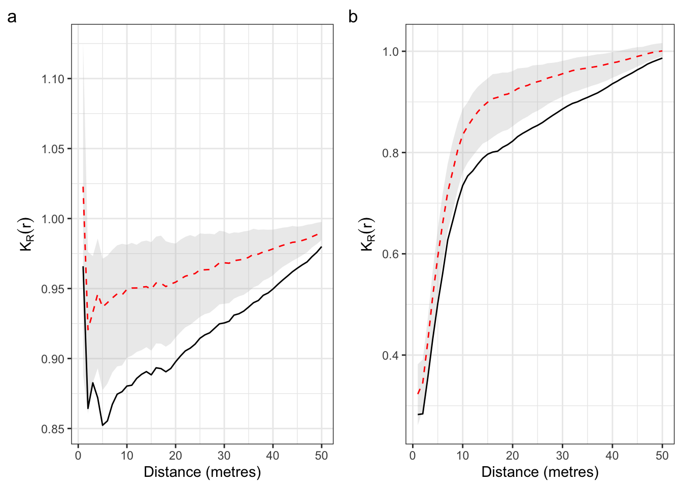
In a first experiment (Figure 1), we simulated habitat preferences by generating heterogeneous spatial patterns in a checked 1-ha plot with two habitats: eight species were simulated with a twofold higher intensity in habitat 1, and 8 species with a twofold higher intensity in habitat 2, so that species abundant in one habitat were rare in the other one. We independently simulated the species-specific spatial patterns as heterogeneous Poisson or heterogeneous Neyman-Scott processes with a Cauchy dispersal kernel (Ghorbani 2013) mimicking dispersal limitation. In the latter, we fixed the scale parameter of the Cauchy kernel at 1, meaning that only 5% of offspring were dispersed beyond 20 m from their mother tree (Munoz et al. 2013). The 16 species-specific patterns were then assembled into multivariate spatial patterns. A hypothetical phylogeny mimicking trait clustering was simulated, where closely-related species have similar habitat preferences (Hardy and Senterre 2007). The cophenetic distances derived from the tree were normalized to 1.
Figure 2 shows that both these patterns exhibit a significant negative departure from the null hypothesis of species equivalence for the same range of \(r\) values that recovers the scale of the phylogenetic spatial structure representing the simulated pattern of habitat preferences.
Limiting similarity
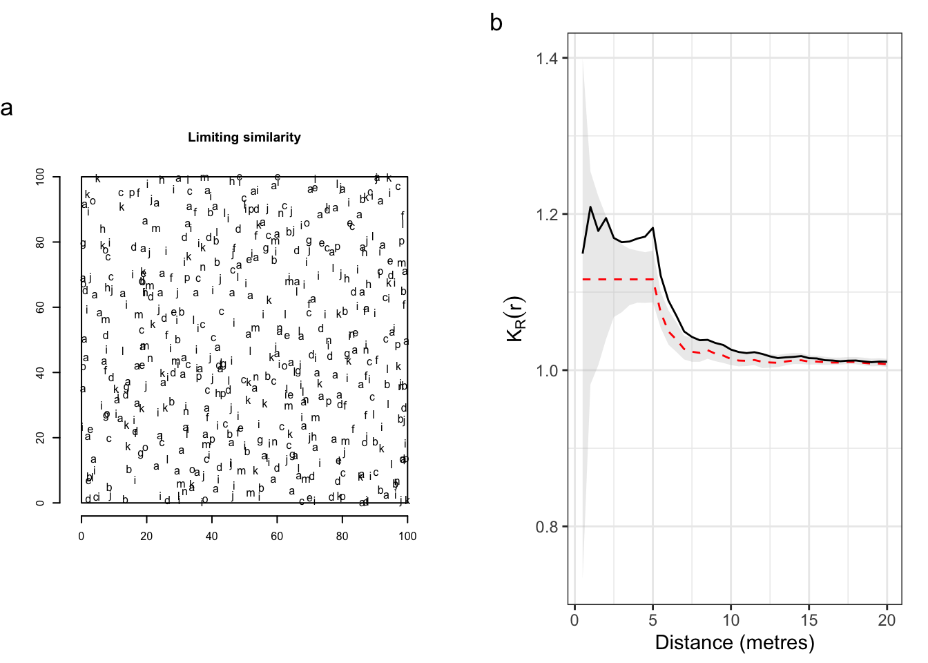
In a second experiment (Figure 3), we simulated a pattern of competitive interaction within a fixed range of 5 m around each individual, using a multitype-Strauss process (Ripley 1988). This point process is defined by an interaction function between each pair of species up to 5 m: \(\phi(r, p, q) = d_{p,q} \leq 1\) if \(r\) < 5 m, \(\phi(r, p, q) = 1\) else. The probability density of a realisation of the point process is proportional to the product of the interaction function applied to all pairs of points: the patterns drawn from the multitype-Strauss process maximize it. Heuristically, spatially close (less than 5 m) pairs of trees reduce the probability of their point pattern compared to more distant pairs if \(d_{p,q} <1\).
This means that the between-species competition intensity within a neighbouring disc of 5 m varies with their proximity within the phylogenetic tree: closely-related species compete more than distantly-related species, with no interaction between species that are not in the same half of the tree because \(d_{p,q} = 1\) in this case.
Figure 3(b) shows that \(K_R(r)\) departs significantly and positively from the null hypothesis of species equivalence for the same range of distances, confirming the limiting similarity pattern originally simulated. Restricted permutations within a cophenetic distance matrix, i.e. between species within clusters or clades in a hierarchical tree, can provide more specific tests of evolutionary hypotheses (Hardy 2008).
3.2 Paracou: a tropical forest plot in French Guiana
Study site and data
We used for application a dataset of tropical forest trees in Paracou experimental station, French Guiana (Gourlet-Fleury et al. 2004). The Paracou experiment was established in 1984 to study the impact of silvicultural treatments on forest dynamics in a series of large (6.25 ha) control and logged plots. We used here data from a control plot (#6) of 250 x 250 m in which 3541 trees with minimum stem diameter at breast height (dbh) of 10 cm were mapped and identified to species level (335 different species). After several scientific programs developed in French Guiana, a database of functional traits is available for the sampled species (Baraloto et al. 2012). For the present application we selected the basic functional traits defining the Leaf-Height-Seed (LHS) scheme of plant strategies (Westoby 1998), i.e. the specific leaf area (SLA in cm2.g-1 of dry matter), the expected tree height at maturity (H in m) and, as a proxy for seed mass, a seed size ordered-codification (Seed), from 1 (very small seeds) to 5 (very big seeds). These traits are acknowledged to illustrate the major trade-offs in plant fitness between resource capture and allocation: SLA characterises the importance of the growth response to favourable conditions, while H and Seed characterise the importance of investment in the capacity to respond to disturbance. We also included the wood specific gravity (WSG in g.cm-3 of dry matter) as a fourth trait specifically accounting for an orthogonal axis (Baraloto et al. 2010) related to additional important functions in trees, such as water transport, structural support, resource storage, defence, etc. (Chave et al. 2009).
From these data, we built two different between-species distance matrices, a phylogenetic one and a functional one based on the four traits described above. The phylogenetic distance was simply computed considering \(d_{p,q} = 1\) if species \(p\) and \(q\) were from the same genus, \(d_{p,q} = 2\) if they were from different genera in the same family and \(d_{p,q} = 3\) if they were from different families. Such a cophenetic distance matrix has ultrametric properties ensuring desirable maximization properties to Rao’s quadratic entropy (Pavoine et al. 2005). The functional distance matrix was based on functional trait dissimilarities, taken as Gower distance (Gower 1971). Its square-root transformation ensured it was Euclidean (Gower 1966), but not ultrametric. Both distance matrices were finally rescaled by their maximum in order to keep Rao’s entropy within the 0-1 standard range of values for diversity indices.
Analysis of species diversity spatial pattern
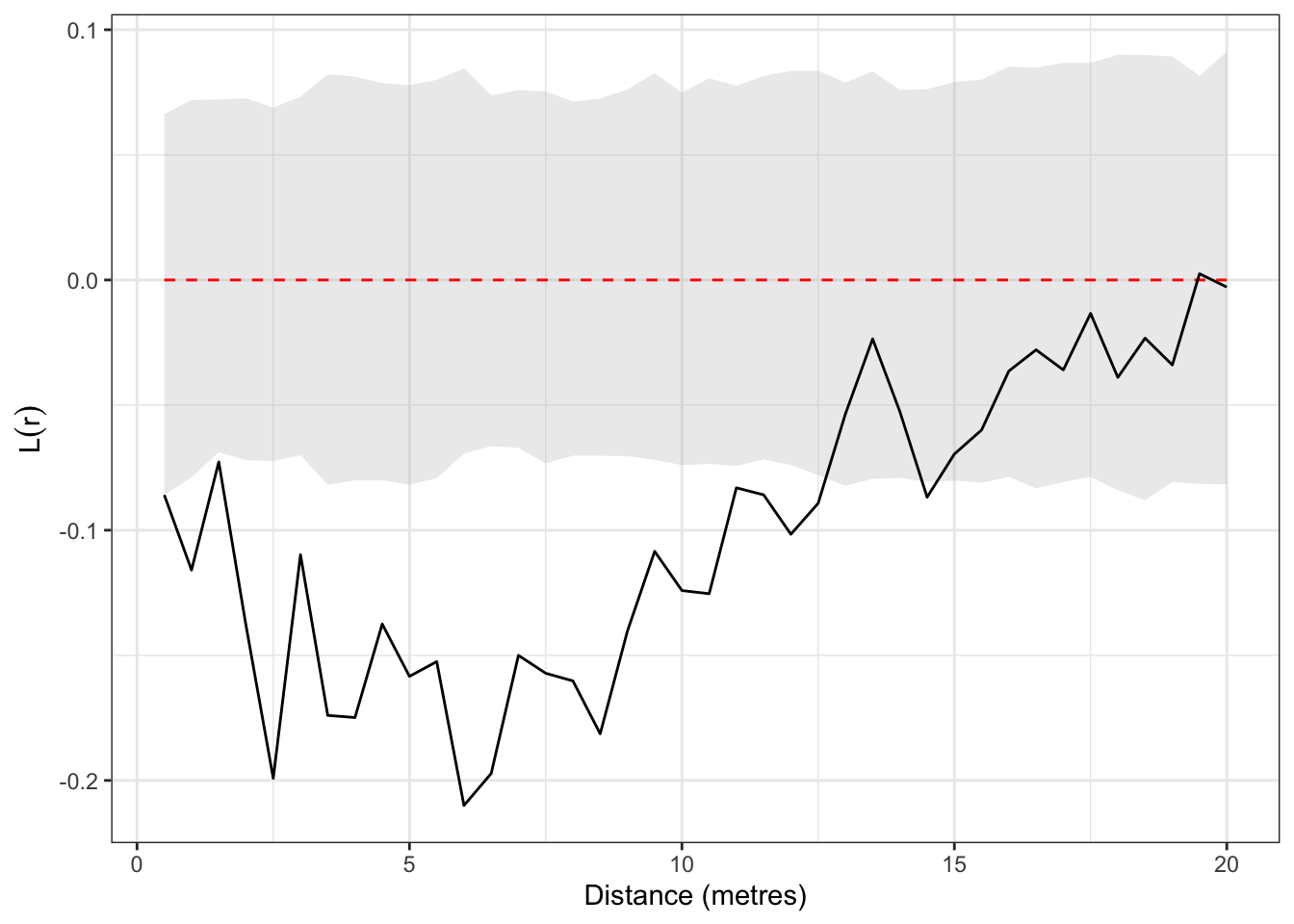
The L-function shows a significant departure towards regularity of the unmarked spatial pattern (i.e. regardless of species labels) up to 12 m (Figure 4).
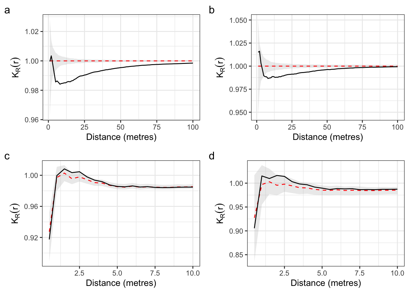
\(K_R(r)\) computed with both phylogenetic and functional between-species distance matrix show very similar patterns (Figure 5). Converging results were expected because the traits retained are generally considered as phylogenetically conserved (e.g. Baraloto et al. 2012).
The random-labelling null hypothesis compares the neighbourhood diversity to that of a plot where the trees are located at the same place but have their species shuffled. Figure 5(a) and (b) show that significantly lower-than-expected diversity occurs up to around 50 m. Habitat preference may be confused with the mere effect of intraspecific aggregation with this null hypothesis.
The species-equivalence null hypothesis preserves the species individual spatial distributions, accounting for intraspecific aggregation. Figure 5(c) and (d) illustrate that under this model we observe higher-than-expected diversity at short distances. The departure from the 1%-confidence envelope of the phylogenetic entropy is not sharp: the curves overlap with the edges of the envelopes.
Short-range spatial regularity in tree stands is generally interpreted to result from self-thinning due to intense local competition (e.g. Kenkel 1988). It therefore seems that the sharing of resources between locally competing neighbours enhanced niche differentiation and thus species diversity. In other words, combining the spatial pattern of diversity (Figure 5) and the spatial pattern of the trees (Figure 4) reveals that limiting similarity in the trees’ neighbourhood drives assembly at small spatial scales. Even though their global point pattern shows regularity at this scale, most tree species are individually aggregated in Paracou (Collinet 1997), and more generally in tropical forests (Condit et al. 2000). Controlling for their spatial structure with the species-equivalence null hypothesis allows for the disentangling of processes that drive the spatial distribution of species.
4 Conclusion
The function of multitype point pattern analysis \(K_R(r)\) introduced here is a normalised version of Rao’s entropy measured in the neighbourhood of individuals.
It relies on two well-known analytical frameworks: the spatial point pattern analysis popularized by Ripley (1977) through his K-function, and the quadratic entropy introduced by Rao (1982) as a diversity coefficient accounting for non-uniform between-species distances. It follows that a spatially continuous and unbiased measure of species diversity can be envisioned as a simple wrapper of classical functions of point pattern analysis, namely the K- and Kp,q-functions. Introducing a non-uniform between-species distance matrix in the quantification of species diversity also provides opportunities to consider different and potentially complementary metrics, based on either taxonomic, phylogenetic or functional differences between species. We note that orthogonal functional axes can also be considered independently using this approach, allowing the potential comparison of assembly processes due to habitat filtering, competition, or interactions with natural enemies. This approach is allowed only by Rao’s entropy, thanks to its mathematical properties: the average distance between individuals relies on the number of pairs of heterospecific individuals, which is straightforwardly linked to the average number of heterospecific individuals summarized by the intertype Kp,q-functions (Equation 8). Other measures of neighbourhood diversity address more aspects of biodiversity but loose link with the point process theory.
Observed spatial diversity patterns can be tested against the highly meaningful ecological hypothesis of species equivalence emphasized by the neutral theory of biodiversity (Hubbell 2001) with the \(K_R(r)\) function. This tool provides a powerful and robust tool to detect significant trait clustering or divergence expected to arise in ecological communities under the driving forces of habitat preferences or local competitive interactions.
References
Altieri, Linda, Daniela Cocchi, and Giulia Roli. 2021. ‘Spatial Entropy for Biodiversity and Environmental Data: The R-Package SpatEntropy’. Environmental Modelling & Software 144 (October): 105149. https://doi.org/10.1016/j.envsoft.2021.105149.
Baraloto, Christopher, Olivier J. Hardy, C. E. Timothy Paine, et al. 2012. ‘Using Functional Traits and Phylogenetic Trees to Examine the Assembly of Tropical Tree Communities’. Journal of Ecology 100 (3): 690–701. https://doi.org/10.1111/j.1365-2745.2012.01966.x.
Baraloto, Christopher, C. E. Timothy Paine, Lourens Poorter, et al. 2010. ‘Decoupled Leaf and Stem Economics in Rain Forest Trees’. Ecology Letters 13 (11): 1338–47. https://doi.org/10.1111/j.1461-0248.2010.01517.x.
Batty, Michael. 1974. ‘Spatial Entropy’. Geographical Analysis 6 (1): 1–31. https://doi.org/10.1111/j.1538-4632.1974.tb01014.x.
Besag, Julian E. 1977. ‘Comments on Ripley’s Paper’. Journal of the Royal Statistical Society: Series B (Statistical Methodology) 39 (2): 193–95. https://doi.org/10.1111/j.2517-6161.1977.tb01616.x.
Cadotte, Marc W., Russel Dinnage, and David Tilman. 2012. ‘Phylogenetic Diversity Promotes Ecosystem Stability’. Ecology 93 (8): S223–33. https://doi.org/10.1890/11-0426.1.
Chao, Anne. 1984. ‘Nonparametric Estimation of the Number of Classes in a Population’. Scandinavian Journal of Statistics 11 (4): 265–70. https://www.jstor.org/stable/4615964.
Chao, Anne, Nicholas J. Gotelli, T. C. Hsieh, et al. 2014. ‘Rarefaction and Extrapolation with Hill Numbers: A Framework for Sampling and Estimation in Species Diversity Studies’. Ecological Monographs 84 (1): 45–67. https://doi.org/10.1890/13-0133.1.
Chave, Jérôme, David Coomes, Steven Jansen, Simon L. Lewis, Nathan G. Swenson, and Amy E. Zanne. 2009. ‘Towards a Worldwide Wood Economics Spectrum’. Ecology Letters 12 (4): 351–66. https://doi.org/10.1111/j.1461-0248.2009.01285.x.
Chave, Jérôme, and Egbert G. Leigh. 2002. ‘A Spatially Explicit Neutral Model of \(\beta\)-Diversity in Tropical Forests’. Theoretical Population Biology 62 (2): 153–68. https://doi.org/10.1006/tpbi.2002.1597.
Clark, James S., David Bell, Chengjin Chu, et al. 2010. ‘High-Dimensional Coexistence Based on Individual Variation: A Synthesis of Evidence’. Ecological Monographs 80 (4): 569–608. https://doi.org/10.1890/09-1541.1.
Collinet, Frédérique. 1997. ‘Essai de Regroupement Des Principales Espèces Structurantes d’une Forêt Dense Humide d’après Leur Répartition Spatiale (Forêt de Paracou, Guyane)’. PhD thesis, Université Claude Bernard, Lyon I.
Condit, Richard, Peter S. Ashton, Patrick Baker, et al. 2000. ‘Spatial Patterns in the Distribution of Tropical Tree Species’. Science 288 (5470): 1414–18. https://doi.org/10.1126/science.288.5470.1414.
Cornwell, William K., Dylan W. Schwilk, and David D. Ackerly. 2006. ‘A Trait-Based Test for Habitat Filtering: Convex Hull Volume’. Ecology 87 (6): 1465–71. https://doi.org/10.1890/0012-9658(2006)87[1465:ATTFHF]2.0.CO;2.
Dale, Mark R. T. 1999. Spatial Pattern Analysis in Plant Ecology. Cambridge Studies in Ecology. Cambridge Univ. Press.
Diggle, Peter J. 1979. ‘On Parameter Estimation and Goodness-of-Fit Testing for Spatial Point Patterns’. Biometrics 35 (1): 87. https://doi.org/10.2307/2529938.
Diggle, Peter J. 1983. Statistical Analysis of Spatial Point Patterns. Academic Press.
Eckel, S., F. Fleischer, P. Grabarnik, and V. Schmidt. 2008. ‘An Investigation of the Spatial Correlations for Relative Purchasing Power in Baden-Wurttemberg’. Asta-Advances in Statistical Analysis 92 (2): 135–52. https://doi.org/10.1007/s10182-008-0066-1.
Ghorbani, Mohammad. 2013. ‘Cauchy Cluster Process’. Metrika 76 (5): 697–706. https://doi.org/10.1007/s00184-012-0411-y.
Goreaud, François, and Raphaël Pélissier. 1999. ‘On Explicit Formulas of Edge-Effect Correction for Ripley’s K-Function’. Journal of Vegetation Science 10 (3): 433–38.
Goreaud, François, and Raphaël Pélissier. 2003. ‘Avoiding Misinterpretation of Biotic Interactions with the Intertype K12 Function: Population Independence Vs Random Labelling Hypotheses’. Journal of Vegetation Science 14 (5): 681–92. https://doi.org/10.1111/j.1654-1103.2003.tb02200.x.
Gotelli, Nicholas J., and Robert K. Colwell. 2001. ‘Quantifying Biodiversity: Procedures and Pitfalls in the Measurement and Comparison of Species Richness’. Ecology Letters 4 (4): 379–91. https://doi.org/10.1046/j.1461-0248.2001.00230.x.
Gourlet-Fleury, Sylvie, Jean Marc Guehl, and Olivier Laroussinie. 2004. Ecology & Management of a Neotropical Rainforest. Lessons Drawn from Paracou, a Long-Term Experimental Research Site in French Guiana. Elsevier.
Gower, J. C. 1966. ‘Some Distance Properties of Latent Root and Vector Methods Used in Multivariate Analysis’. Biometrika 53 (3): 325–38. https://doi.org/10.1093/biomet/53.3-4.325.
Gower, J. C. 1971. ‘A General Coefficient of Similarity and Some of Its Properties’. Biometrics 27 (4): 857–71. https://doi.org/10.2307/2528823.
Hardy, Olivier J. 2008. ‘Testing the Spatial Phylogenetic Structure of Local Communities: Statistical Performances of Different Null Models and Test Statistics on a Locally Neutral Community’. Journal of Ecology 96 (5): 914–26. https://doi.org/10.1111/j.1365-2745.2008.01421.x.
Hardy, Olivier J., and Bruno Senterre. 2007. ‘Characterizing the Phylogenetic Structure of Communities by an Additive Partitioning of Phylogenetic Diversity’. Journal of Ecology 95 (3): 493–506. https://doi.org/10.1111/j.1365-2745.2007.01222.x.
Hubbell, Stephen P. 2001. The Unified Neutral Theory of Biodiversity and Biogeography. Princeton University Press.
Hubbell, Stephen P., Jorge A. Ahumada, Richard Condit, and Robin B. Foster. 2001. ‘Local Neighborhood Effects on Long-Term Survival of Individual Trees in a Neotropical Forest’. Ecological Research 16 (5): 859–75. https://doi.org/10.1046/j.1440-1703.2001.00445.x.
Jost, Lou. 2006. ‘Entropy and Diversity’. Oikos 113 (2): 363–75. https://doi.org/10.1111/j.2006.0030-1299.14714.x.
Jost, Lou. 2007. ‘Partitioning Diversity into Independent Alpha and Beta Components’. Ecology 88 (10): 2427–39. https://doi.org/10.1890/06-1736.1.
Jurasinski, Gerald, Vroni Retzer, and Carl Beierkuhnlein. 2009. ‘Inventory, Differentiation, and Proportional Diversity: A Consistent Terminology for Quantifying Species Diversity’. Oecologia 159 (1): 15–26. https://doi.org/10.1007/s00442-008-1190-z.
Keddy, P. A. 1992. ‘A Pragmatic Approach to Functional Ecology’. Functional Ecology 6 (6): 621. https://doi.org/10.2307/2389954.
Kenkel, N. C. 1988. ‘Pattern of Self-Thinning in Jack Pine: Testing the Random Mortality Hypothesis’. Ecology 69 (4): 1017–24. https://doi.org/10.2307/1941257.
Lande, Russell. 1996. ‘Statistics and Partitioning of Species Diversity, and Similarity Among Multiple Communities’. Oikos 76 (1): 5–13. https://doi.org/10.2307/3545743.
Losos, Elizabeth C., and Egbert Giles Leigh. 2004. Tropical Forest Diversity and Dynamism: Findings from a Large-Scale Plot Network. University of Chicago press.
Lotwick, H. W., and B. W. Silverman. 1982. ‘Methods for Analysing Spatial Processes of Several Types of Points’. Journal of the Royal Statistical Society: Series B (Statistical Methodology) 44 (3): 406–13. https://www.jstor.org/stable/2345499.
MacArthur, Robert H., and Richard Levins. 1967. ‘The Limiting Similarity, Convergence, and Divergence of Coexisting Species’. The American Naturalist 101 (921): 377–85. https://doi.org/10.1086/282505.
Marcon, Eric, and Bruno Hérault. 2015. ‘Decomposing Phylodiversity’. Methods in Ecology and Evolution 6 (3): 333–39. https://doi.org/10.1111/2041-210X.12323.
Marcon, Eric, and Florence Puech. 2026. Divent: Entropy Partitioning to Measure Diversity. Manual. https://doi.org/10.32614/CRAN.package.divent.
Marcon, Eric, Ivan Scotti, Bruno Hérault, Vivien Rossi, and Gabriel Lang. 2014. ‘Generalization of the Partitioning of Shannon Diversity’. Plos One 9 (3): e90289. https://doi.org/10.1371/journal.pone.0090289.
Marcon, Eric, Stéphane Traissac, Florence Puech, and Gabriel Lang. 2015. ‘Tools to Characterize Point Patterns: dbmss for R’. Journal of Statistical Software 67 (3): 1–15. https://doi.org/10.18637/jss.v067.c03.
Mouquet, Nicolas, Vincent Devictor, Christine N. Meynard, et al. 2012. ‘Ecophylogenetics: Advances and Perspectives’. Biological Reviews 87 (4): 769–85. https://doi.org/10.1111/j.1469-185X.2012.00224.x.
Munoz, François, Champak R. Beeravolu, Raphaël Pélissier, and Pierre Couteron. 2013. ‘Do Spatially-Implicit Estimates of Neutral Migration Comply with Seed Dispersal Data in Tropical Forests?’ Plos One 8 (8). https://doi.org/10.1371/journal.pone.0072497.
Nemetschek, Daniela, Claire Fortunel, Eric Marcon, et al. 2025. ‘Love Thy Neighbour? Tropical Tree Growth and Its Response to Climate Anomalies Is Mediated by Neighbourhood Hierarchy and Dissimilarity in Carbon- and Water-Related Traits’. Ecology Letters 28 (4): e70028. https://doi.org/10.1111/ele.70028.
Pavoine, Sandrine. 2012. ‘Clarifying and Developing Analyses of Biodiversity: Towards a Generalisation of Current Approaches’. Methods in Ecology and Evolution 3 (3): 509–18. https://doi.org/10.1111/j.2041-210X.2011.00181.x.
Pavoine, Sandrine, and Michael B. Bonsall. 2011. ‘Measuring Biodiversity to Explain Community Assembly: A Unified Approach’. Biological Reviews 86 (4): 792–812. https://doi.org/10.1111/j.1469-185X.2010.00171.x.
Pavoine, Sandrine, Anne-Béatrice Dufour, and Daniel Chessel. 2004. ‘From Dissimilarities Among Species to Dissimilarities Among Communities: A Double Principal Coordinate Analysis’. Journal of Theoretical Biology 228 (4): 523–37. https://doi.org/10.1016/j.jtbi.2004.02.014.
Pavoine, Sandrine, Sébastien Ollier, and D. Pontier. 2005. ‘Measuring Diversity from Dissimilarities with Rao’s Quadratic Entropy: Are Any Dissimilarities Suitable?’ Theoretical Population Biology 67 (4): 231–39. https://doi.org/10.1016/j.tpb.2005.01.004.
Pavoine, Sandrine, Errol Vela, Sophie Gachet, Gérard de Belair, and Michael B. Bonsall. 2011. ‘Linking Patterns in Phylogeny, Traits, Abiotic Variables and Space: A Novel Approach to Linking Environmental Filtering and Plant Community Assembly’. Journal of Ecology 99 (1): 165–75. https://doi.org/10.1111/j.1365-2745.2010.01743.x.
Pélissier, Raphaël, and François Goreaud. 2015. ‘Ads Package for R: A Fast Unbiased Implementation of the K -Function Family for Studying Spatial Point Patterns in Irregular-Shaped Sampling Windows’. Journal of Statistical Software 63 (6): 1–18. https://doi.org/10.18637/jss.v063.i06.
Picard, Nicolas, M. Karembe, and Philippe Birnbaum. 2004. ‘Species-Area Curve and Spatial Pattern’. Ecoscience 11 (1): 45–54. https://doi.org/10.1080/11956860.2004.11682808.
Pielou, Evelyn C. 1975. Ecological Diversity. Wiley.
R Core Team. 2026. R: A Language and Environment for Statistical Computing. R Foundation for Statistical Computing.
Rajala, T., and J. Illian. 2012. ‘A Family of Spatial Biodiversity Measures Based on Graphs’. Environmental and Ecological Statistics 19 (4): 545–72. https://doi.org/10.1007/s10651-012-0200-9.
Rao, C. Radhakrishna. 1982. ‘Diversity and Dissimilarity Coefficients: A Unified Approach’. Theoretical Population Biology 21 (1): 24–43. https://doi.org/10.1016/0040-5809(82)90004-1.
Ripley, Brian D. 1976. ‘The Second-Order Analysis of Stationary Point Processes’. Journal of Applied Probability 13 (2): 255–66. https://doi.org/10.2307/3212829.
Ripley, Brian D. 1977. ‘Modelling Spatial Patterns’. Journal of the Royal Statistical Society: Series B (Statistical Methodology) 39 (2): 172–212. https://doi.org/10.1111/j.2517-6161.1977.tb01615.x.
Ripley, Brian D. 1988. Statistical Inference for Spatial Processes. Cambridge University Press. https://doi.org/10.1017/CBO9780511624131.
Shen, Guochun, Thorsten Wiegand, Xiangcheng Mi, and Fangliang He. 2013. ‘Quantifying Spatial Phylogenetic Structures of Fully Stem-Mapped Plant Communities’. Methods in Ecology and Evolution 4 (12): 1132–41. https://doi.org/10.1111/2041-210X.12119.
Shimatani, Kenichiro. 2001a. ‘Multivariate Point Processes and Spatial Variation of Species Diversity’. Forest Ecology and Management 142 (1-3): 215–29. https://doi.org/10.1016/s0378-1127(00)00352-2.
Shimatani, Kenichiro. 2001b. ‘On the Measurement of Species Diversity Incorporating Species Differences’. Oikos 93 (1): 135–47. https://doi.org/10.1034/j.1600-0706.2001.930115.x.
Simpson, Edward H. 1949. ‘Measurement of Diversity’. Nature 163 (4148): 688. https://doi.org/10.1038/163688a0.
Stoyan, Dietrich, W. S. Kendall, and Joseph Mecke. 1987. ‘Stochastic Geometry and Its Applications’. In Wiley Series in Probability and Mathematical Statistics. John Wiley & Sons.
Ugland, Karl I., John S. Gray, and Kari E. Ellingsen. 2003. ‘The Species-Accumulation Curve and Estimation of Species Richness’. Journal of Animal Ecology 72 (5): 888–97. https://doi.org/10.1046/j.1365-2656.2003.00748.x.
Webb, Campbell O., David D. Ackerly, Mark A. McPeek, and Michael J. Donoghue. 2002. ‘Phylogenies and Community Ecology’. Annual Review of Ecology and Systematics 33: 475–505. https://doi.org/10.1146/annurev.ecolsys.33.010802.150448.
Westoby, Mark. 1998. ‘A Leaf-Height-Seed (LHS) Plant Ecology Strategy Scheme’. Plant and Soil 199: 213–27. https://doi.org/10.1023/A:1004327224729.
Whittaker, R. H. 1960. ‘Vegetation of the Siskiyou Mountains, Oregon and California’. Ecological Monographs 30 (3): 279–338. https://doi.org/10.2307/1943563.
Wiegand, Thorsten, and Kirk A. Moloney. 2004. ‘Rings, Circles, and Null-Models for Point Pattern Analysis in Ecology’. Oikos 104 (2): 209–29. https://doi.org/10.1111/j.0030-1299.2004.12497.x.
Wiegand, Thorsten, María Uriarte, Nathan J. B. Kraft, Guochun Shen, Xugao Wang, and Fangliang He. 2017. ‘Spatially Explicit Metrics of Species Diversity, Functional Diversity, and Phylogenetic Diversity: Insights into Plant Community Assembly Processes’. Annual Review of Ecology, Evolution, and Systematics 48 (1): 329–51. https://doi.org/10.1146/annurev-ecolsys-110316-022936.